Il y a un mouvement si le vecteur ![]() change au fil du temps. On peut donc noter cette dépendance
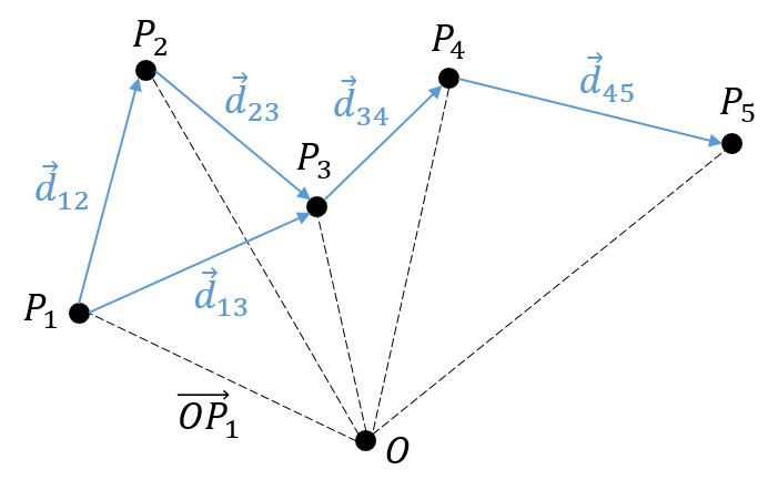
change au fil du temps. On peut donc noter cette dépendance ![]() . La variation de la position est ce mouvement. En connaissant la position de l’objet P1, P2, P3, …à des moments consécutifs t1, t2, t3, … ,nous pouvons introduire le vecteur de déplacement
. La variation de la position est ce mouvement. En connaissant la position de l’objet P1, P2, P3, …à des moments consécutifs t1, t2, t3, … ,nous pouvons introduire le vecteur de déplacement ![]() comme le vecteur
comme le vecteur ![]() , et si l’objet continue à bouger,
, et si l’objet continue à bouger, ![]() , etc.
, etc.
Plusieurs observations peuvent être faites à ce stade:
- la position
 est l’ addition de la position précédente
  avec le déplacement
  .
.
![]()
- le déplacement
 est égale à la somme des déplacements et
  .
.
![]()
- cela peut sembler évident, mais il faut savoir que le nombre de positions est toujours plus que le nombre de déplacements. En conséquence, il est impossible de déterminer la position de l’objet à partir de ses seuls déplacements. Nous aurons besoin d’au moins une de ses positions.
Nous avons présenté ici l’opérateur d’addition + sur les vecteurs. Dans le système cartésien, il est facile de voir que les opérateurs d’addition et de soustraction sont simplement les opérateurs mathématiques + et – appliqués sur les nombres correspondant aux coordonnées.

La vitesse moyenne :
Maintenant que les déplacements sont définis, on peut considérer que le temps pour faire le déplacement entre P1 et P5 directement n’est pas le même que si on le fait avec des étapes intermédiaires. La vitesse moyenne est le déplacement moyen en unité de temps. Au temps t1, l’objet se trouvait en position P1 définit par le vecteur de position. Au temps t2, l’objet s’est déplacé à la position P2, définit par le vecteur de position. La vitesse moyenne entre ces deux positions est donc le déplacement de l’objet divisé par l’intervale de temps t2-t1.
![]()
La vitesse est dite moyenne car elle dépend des deux positions choisies. Une notation courante en mathématiques consiste à écrire les différences de deux valeurs par le signe Δ. Nous pouvons donc écrire
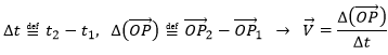
Que nous pouvons aussi écrire, avec la dépendance explicite sur le temps:
![]()
The instantaneous speed
One concept is now to get rid of the two positions to define an instantaneous speed, associated to a given position and a given time. To do so, we will bring the second point closer from the first and see what happens. We can’t only chose one point because the division by zero is not allowed. However, if this ratio continues to exist when the two points are almost identical, then the instantaneous speed is this value.
![]()
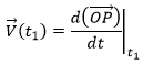
It is also the definition of the derivative of the position with regards to the time, calculated at t1. The limit towards zero of Δ will be noted d to obtain the notation corresponding to the usual derivative.
![]()
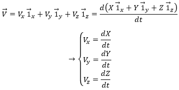
To indicate at which time we look for the speed, we use the notation
Each component of the speed is given by the derivative of the corresponding component of the position with regards to the time.
The acceleration
The same way we defined the speed as the variation of the position over time, the acceleration a is the variation of speed over time. We define an average acceleration as
![]()
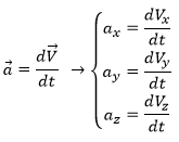
and the instantaneous acceleration as the derivative of the speed vector with regards to the time.
The acceleration can be obtained directly from the position by taking its second derivative. We introduce the notations
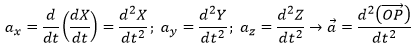
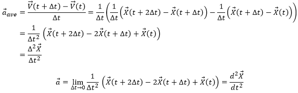
Note the difference of position of the square exponent: it is the derivative d/dt that is taken twice, not the object of the derivative. It is more evident if we use the definition of the derivative explicitly:
From acceleration to speed
As the acceleration is a difference of speed, there is thus always one acceleration less than there are speeds. From a speed at a time t1, on can determine the speed at a time t2 if we are given the acceleration during the interval of time.
![]()
From point to point, we can thus determine the speed:
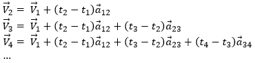
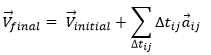
We can generalise this as
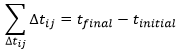
Obviously, the sum of the intervals of times equals the elapsed time:
At the limit of the discrete time jumps, the sum becomes an integration
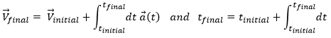
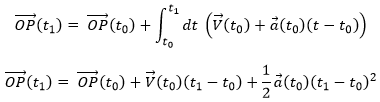
From the speed to the position
We can apply the same method on the speed to obtain the position:
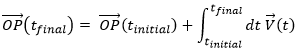
Let insist on the physical meaning of this:
- the integration∫ is a sum,
- this sum is always made on a product,
- this product always contain an infinitesimal difference (here the time dt) and one finite quantity (here the speed V(t)),
- the sum ∫ is defined between a point of beginning and a point of end.
The uniform rectilinear motion
A uniform rectilinear motion (URM) is obtained when the speed of the object doesn’t depend upon time. The speed is thus constant and is defined at the initial time t0.
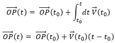
As the speed is constant, the acceleration is thus zero.
![]()
The equations for the position in each direction correspond to the equation of a straight line in the three dimensions space.
![]()
The uniformly accelerated rectilinear motion
Another simple problem is when the acceleration is constant. Similarly to the URM, here we easily find the speed:
![]()
And the position: