Nouveau Traitement de l’hypertension par remodelage du système nerveux autonome
Nouveau Traitement de l’hypertension
Le remodelage du système nerveux autonome par rééducation limbique est une technique très sophistiquée permettant un traitement physiologique de l’hypertension artérielle sans aucun médicament (si la procédure est appliquée aux premiers stades de la maladie). En cas d’hypertension très ancienne, le traitement prendra plusieurs mois en raison des anomalies secondaires à action prolongée de la tension sur les organes (hypertrophie myocardique et une augmentation de la résistance vasculaire aussi secondaire à une hypertrophie musculaire des parois ainsi qu’un processus hormonal et humoral réactionnel très actif). Pour comprendre l’efficacité de cette technique, nous devons commencer à étudier l’étiologie et le mécanisme exact conduisant à l’hypertension
Physiopathologie de l’Hypertension artérielle :
L’hypertension artérielle est une cause majeure de morbidité et de mortalité en raison de son association avec les maladies coronariennes, les maladies cérébro-vasculaires et les maladies rénales. L’étendue de l’atteinte des organes cibles (c.à.d. le cœur, le cerveau et les reins) détermine le pronostic. Selon O.M.S (organisation mondiale de la santé) Chaque année, 15 millions de personnes font un A.V.C et 5 millions d’ente elles meurent et 5 millions souffrent d’une incapacité permanente. L’A.V.C est rare chez les moins de 40 ans et s’il survient, c’est principalement à cause de l’HTA . L’hypertension et le tabagisme sont les deux grands facteurs de risque modifiables. Sur dix personnes décédés d’un AVC, quatre aurait pu être sauvées si leur tension avait été maîtrisée. Des directives récentes, indiquent clairement que le traitement de l’hypertension systolique isolée est aussi important que celui de l’hypertension systolo-diastolique.
Les différents niveaux de la tension artérielle selon OMS :
Elevé : Ts : > ou = 140 mm Hg et Td : > ou = 90 mmHg
à risque (préhypertension) : Ts : 120-139 mm Hg et Td : 80-89 mm Hg
Normal : Ts < 120 mm Hg et Td : < 80 à 85 mm Hg
La tension artérielle est déterminée par 3 éléments fondamentaux :
Volume d’éjection ventriculaire gauche , Fréquence cardiaque et la résistance vasculaire périphérique
PA = VES x frc x RVP
Ce qui est égale à débit cardiaque x résistance vasculaire périphérique.
Le rôle du système nerveux sympathique dans l’Hypertension artérielle:
En 1988: Vargas HM, Brezenoff HE. ont démontré la supression de l’hypertension lors de la réduction chronique de l’acétylcholine cérébrale chez les rats spontanément hypertendus. Journal of Hypertension. 1988; 6 (9): 739–745. Des expériences ont été menées pour déterminer les effets de l’épuisement chronique de l’acétylcholine cérébrale (ACh) sur le développement et le maintien de l’hypertension chez les rats spontanément hypertendus (RSH). La synthèse de l’ACh cérébrale a été inhibée par la perfusion chronique d’hémicholinium-3 (HC-3) dans les ventricules cérébraux, et la pression artérielle systolique a été surveillée par occlusion de la queue par la coiffe. Chez les RSH de 18 semaines, la perfusion de HC-3 (0,25 microgrammes / h) a supprimé le développement de l’hypertension par rapport aux RSH témoins infusés de solution saline au cours des 21 jours de perfusion (140 contre 190 mm Hg au 21e jour). L’ACh hypothalamique et du tronc cérébral au cours de cette période a été réduit respectivement de 50% et de 60 à 75%. Dans les RSH de 18 semaines avec une hypertension établie, HC-3 (0,25 et 0,5 microgrammes / h) a réduit la pression artérielle systolique de 35 à 40 mm Hg pendant 8 jours, après quoi les pressions sont revenues au niveau de contrôle (191 mm Hg) au jour 14 L’augmentation de la pression artérielle s’est accompagnée d’une récupération des taux hypothalamiques d’ACh à 75% du contrôle. La spécificité et l’efficacité physiologique du HC-3 ont été démontrées par sa capacité à inhiber la réponse pressive médiée centralement à la physostigmine mais pas à l’oxotrémorine. La perfusion de HC-3 n’a pas affecté la croissance corporelle, la consommation d’eau, la température corporelle ou le comportement brut. De cette étude, on peut conclure que les neurones cholinergiques cérébraux sont un élément important dans le développement et le maintien de l’hypertension chez le RSH.
En 1991 : Julius S. Autonomic nervous system dysregulation in human hypertension. American Journal of Cardiology. 1991;67(10):3B–7B
Une augmentation de l’activité sympathique combinée à une diminution de l’inhibition parasympathique est observée chez les patients souffrant d’hypertension borderline, qui ont généralement un rythme cardiaque rapide, un débit cardiaque élevé et une résistance vasculaire relativement normale (état hyperkinétique). Dans l’hypertension établie, le débit cardiaque est normal, la résistance vasculaire est élevée et les signes d’augmentation de l’activité sympathique sont absents. Apparemment, l’hémodynamique et l’activité sympathique changent pendant l’hypertension. Le mécanisme de la transition hémodynamique au cours de l’hypertension est bien connu.
Le débit cardiaque revient des valeurs élevées à normales à mesure que les récepteurs bêta-adrénergiques régulent à la baisse et que le volume systolique diminue (en raison d’une diminution de la compliance cardiaque). L’hypertension artérielle induit une hypertrophie vasculaire, qui à son tour conduit à une résistance vasculaire accrue.
Le mécanisme du changement de tonus sympathique d’une hypertension limite élevée à une hypertension apparemment normale peut être mieux expliqué dans le cadre conceptuel des propriétés de « recherche de la pression artérielle » du cerveau. Dans l’hypertension, le système nerveux central cherche à maintenir la pression artérielle systémique au niveau supérieur.À mesure que l’hypertension progresse et que l’hypertrophie vasculaire se développe, les artérioles deviennent hyper-sensibles à la vasoconstriction. À ce stade, moins d’activité sympathique est nécessaire pour maintenir une vasoconstriction élévatrice de pression, et l’activité sympathique centrale est régulée à la baisse. L’étiologie de l’activité sympathique accrue dans l’hypertension reste non résolue.
Les sujets avec une poussée sympathique accrue sont également généralement en surpoids et ont des niveaux élevés d’insuline, de cholestérol et de triglycérides, ainsi qu’une diminution des lipoprotéines de haute densité. Les recherches futures doivent se concentrer sur le lien entre les facteurs de risque coronariens et l’hyperactivité sympathique dans l’hypertension.
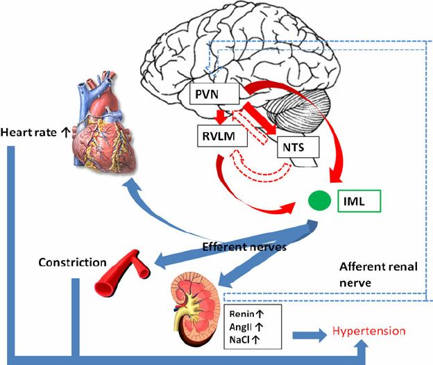
En 2012, Takao Saruta & co a montré l’importance des neurones dans la région RVLM (rostral ventrolateral medulla) et un cercle vicieux entre le SNS (système nerveux sympathique) et le RAS (système rénine-angiotensine) dans la régulation du SNA périphérique, en utilisant la technique patch-clamp à cellules entières. L’imagerie optique a démontré qu’une colonne céphalo-caudale longitudinale dans la moelle ventrolatérale peut réguler le SNS et la PA et a suggéré que:
L’activité nerveuse sympathique accentuée (SNA) induite par les neurones de la médullaire ventrolatérale céphalique (RVLM) est une cause principale d’hypertension essentielle
Comment le systeme nerveux agit?
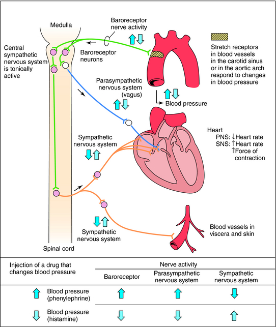
Contrôle aigu des barorécepteurs: Le centre vasomoteur comprend le noyau du tractus solitaire dans la médullaire dorsale (intégration des barorécepteurs), la partie rostrale de la médullaire ventrale (région de pression) et d’autres centres dans les pons et le mésencéphale. Les barorécepteurs artériels répondent à la distension de la paroi vasculaire en augmentant l’activité impulsionnelle afférente. Cela diminue à son tour l’activité sympathique efférente et augmente le tonus vagal. L’effet net est la bradycardie et la vasodilatation.
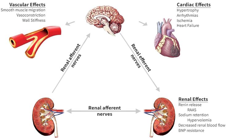
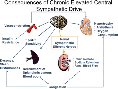
conséquences d’une hyperactivité sympathique prolongée
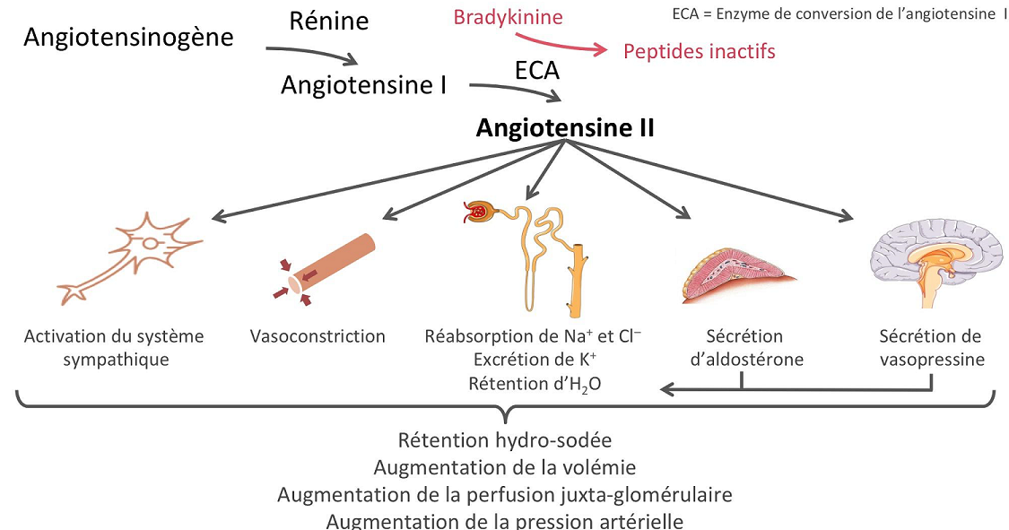
Système rénine-angiotensine :
La rénine protéase clive l’angiotensine pour donner le peptide inactif angiotensine I. Cette dernière est convertie en un octapeptide actif, l’angiotensine II par l’enzyme de conversion de l’angiotensine (ECA). Bien que le système rénine-angiotensine soit répandu dans le corps, la principale source de rénine est l’appareil juxtaglomérulaire du rein. Cet appareil détecte la pression de perfusion rénale et la concentration de sodium dans le liquide tubulaire distal.
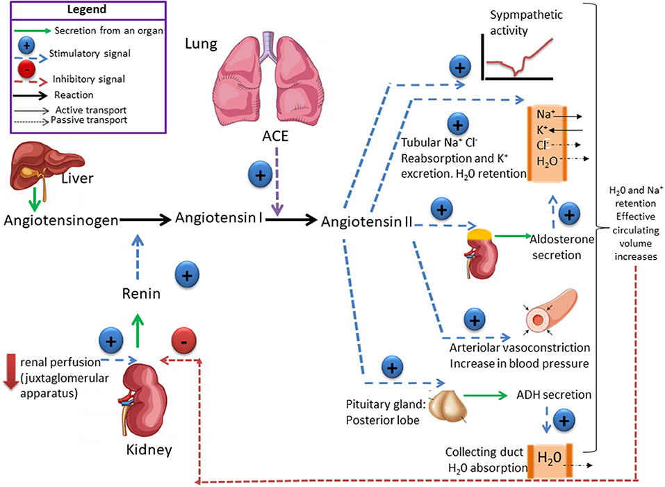
De plus, la libération de rénine est stimulée par le système nerveux sympathique.
Des concentrations élevées d’angiotensine II suppriment la sécrétion de rénine via une boucle de rétroaction négative. L’angiotensine II agit sur des récepteurs spécifiques de l’angiotensine AT1 et AT2, provoquant une contraction des muscles lisses et la libération d’aldostérone, de prostacyclines et des catécholamines. Le système de rénine – angiotensine – aldostérone joue un rôle important dans le contrôle de la pression artérielle, y compris l’équilibre sodique.
ADH ( vasopressin):
Vasopressin is a small hormone, synthesized in the hypothalamus and released into the circulation from the posterior lob of hypophysis. Although historically named as a result of its potent vasopressor actions, these actions only occur when plasma vasopressin is present in the plasma in supraphysiological concentrations. The most important action of vasopressin is its antidiuretic action on the collecting ducts of the kidney. This leads to a decrease in renal free water clearance, concentration of urine, and a reduction in urine volume. The net effect is the reabsorption of water into the blood, which, along with thirst-generated water intake, leads to normalization of plasma osmolality.Regulation of vasopressin secretion and action thus represents a key homeostatic process which protects the osmotic milieu of the body, allowing normal cellular function.
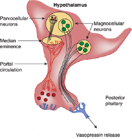
Synthesis :
Vasopressin is most abundantly produced in magnocellular neurosecretory neurons in the supraoptic and paraventricular (PVN) nuclei, transported to terminals in the neurohypophysis, and released into the general circulation. Vasopressin production is also found in parvocellular neurons in the PVN and vasopressinn produced in these neurons is transported to terminals in the external layer of the median eminence, from which it is released into the hypophysial portal system.
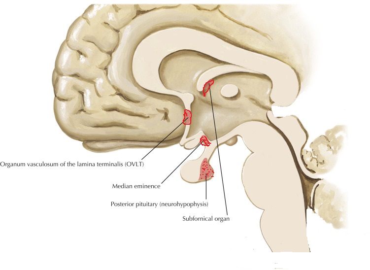
Release and feedback controle :
Vasopressin release is regulated by osmoreceptors in the hypothalamus (OVLT, SFO), which are exquisitely sensitive to changes in plasma osmolality of as little as 1% to 2%. Under hyperosmolar conditions, osmoreceptor stimulation leads to vasopressin release and stimulation of thirst. These two mechanisms result in increased water intake and retention. Vasopressin release is also regulated by baroreceptors in the carotid sinus and aortic arch, under conditions of hypovolemia, these receptors stimulate vasopressin release to increase plasma volume. At very high concentrations, vasopressin also causes vascular smooth muscle constriction through the V1 receptor, increasing vascular tone and therefore the blood pressure. Accordingly, vasopressin is often administered parenterally as a vasopressor agent in patients with hypotension that is refractory to volume restriction.
 Vasopressin has effects on the immune system independent of its effect in stimulating the HPA axis. When given intraventricularly to rats, vasopressin decreases the T-cell response to mitogen independently of the HPA axis, probably via the sympathetic nervous system. Like CRH, vasopressin stimulates immune responses in peripheral tissues. Circulating or local vasopressin enhances lymphocyte reactions and potentiates primary antibody. Elevated vasopressin levels are found in a mouse model of autoimmune disease, and antibody neutralization ameliorates the inflammatory response in these mice. Vasopressin can potentiate the release of prolactin, a proinflammatory peptide hormone.
Because vasopressin has immunosuppressive effects when present in the central nervous system and immunosupportive effects when present in peripheral tissues, predicting which effect would predominate during vasopressin infusion in the ICU is difficult.
Vasopressin is a hormone of the posterior pituitary, that is secreted in response to high serum osmolarity. Excitation of atrial stretch receptors inhibits vasopressin secretion. Vasopressin is also released in response to stress, inflammatory signals, and some medications. Hypotension, morphine, nicotine, angiotensin II, glucocorticoids, and IL-6 all stimulate release of vasopressin. Circulating vasopressin levels are usually high in the early phase of septic shock, but vasopressin deficiency has been described in vasodilatory shock states in both adults and children. The level of vasopressin that is normal in the late phase of sepsis is unclear.
Vasopressin selectively raises free water reabsorption through the upregulation of aquaporin-2 water channels in the collecting duct, resulting in blood pressure elevation (Elliot et al., 1996; Linshaw 2011). Although it appears that the developing kidney is less sensitive to circulating vasopressin, plasma levels of vasopressin are markedly elevated in the neonate, especially after vaginal delivery, and its cardiovascular actions facilitate neonatal adaptation (Pohjavuori et al., 1985; Linshaw, 2011). The high vasopressin levels are in part also responsible for the diminished urine output of the healthy term neonate during the first day after birth. Under certain pathologic conditions, the dysregulated release of, or the end-organ unresponsiveness to, vasopressin significantly affects renal and cardiovascular functions and electrolyte and fluid status in the sick preterm and term neonate (Svenningsen et al., 1974). In the syndrome of inappropriate secretion of antidiuretic hormone (SIADH), an uncontrolled release of vasopressin occurs in sick preterm and term neonates, with resulting water retention, hyponatremia, and oligouria. In the syndrome of diabetes insipidus, the lack of pituitary production of vasopressin or renal unresponsiveness to vasopressin results in polyuria and hypernatremia.
Le Peptide natriurétique auriculaire :
Le peptide natriurétique auriculaire (ANP) est libéré des granules auriculaires. Il produit une natriurèse, une diurèse et une baisse modeste de la pression artérielle, tout en diminuant la rénine et l’aldostérone plasmatiques. Les peptides natriurétiques modifient également la transmission synaptique des osmorécepteurs. Le (PNA) est libéré à la suite de la stimulation de l’oreillette par distension et étirement des récepteurs. Les concentrations de (PNA) sont augmentées par des pressions de remplissage élevées et chez les patients souffrant d’hypertension artérielle et d’hypertrophie ventriculaire gauche comme la paroi du ventricule gauche est épaissie participe à la sécrétion d’ANP.
Eicosanoïdes :
Les métabolites de l’acide arachidonique modifient la pression artérielle par des effets directs sur le tonus musculaire lisse vasculaire et les interactions avec d’autres systèmes vasorégulateurs: système nerveux autonome, le système rénine-angiotensine – aldostérone et autres voies humorales. Chez les patients hypertendus, un dysfonctionnement des cellules endothéliales vasculaires pourrait entraîner une réduction des facteurs de relaxation dérivés de l’endothélium tels que l’oxyde nitrique, la prostacycline et le facteur hyperpolarisant dérivé de l’endothélium, ou une augmentation de la production de facteurs de contraction tels que l’endothéline-1 et le thromboxane A2. Systèmes kallikréine-kinine Les kallikréines tissulaires agissent sur le kininogène pour former des peptides vasoactifs. Le plus important est le bradykinin vasodilatateur. Les kinines jouent un rôle dans la régulation du débit sanguin rénal et de l’excrétion d’eau et de sodium. Les inhibiteurs de l’ECA diminuent la dégradation de la bradykinine en peptides inactifs. Mécanismes endothéliaux L’oxyde nitrique (NO) intervient dans la vasodilatation produite par l’acétylcholine, la bradykinine, le nitroprussiate de sodium et les nitrates. Chez les patients hypertendus, la relaxation dérivée de l’endothélium est inhibée. L’endothélium synthétise les endothélines, les vasoconstricteurs les plus puissants. La génération ou la sensibilité à l’endothéline-1 n’est pas plus élevée chez les sujets hypertendus que chez les sujets normotendus. Néanmoins, les effets vasculaires délétères de l’endothéline-1 endogène peuvent être accentués par une génération réduite d’oxyde nitrique causée par une dysfonction endothéliale hypertensive.
Stéroïdes surrénales :
Les minéraux et glucocorticoïdes augmentent la pression artérielle. Cet effet est médié par la rétention de sodium et d’eau (minéralocorticoïdes) ou une réactivité vasculaire accrue (glucocorticoïdes). De plus, les glucocorticoïdes et les minéralocorticoïdes augmentent le tonus vasculaire en régulant les récepteurs des hormones pressives telles que l’angiotensine II. Vasodépression rénomédullaire Les cellules interstitielles rénomédullaires, situées principalement dans la papille rénale, sécrètent une substance inactive la médullipine I. Ce lipide est transformé dans le foie en médullipine II. Cette substance exerce un effet hypotenseur prolongé, éventuellement par vasodilatation directe, inhibition de la pulsion sympathique en réponse à l’hypotension et une action diurétique. On suppose que l’activité du système rénomédullaire est contrôlée par le flux sanguin médullaire rénal. Excrétion de sodium et d’eau La rétention de sodium et d’eau est associée à une augmentation de la pression artérielle. Il est postulé que le sodium, via le mécanisme d’échange sodium-calcium, provoque une augmentation du calcium intracellulaire dans le muscle lisse vasculaire entraînant une augmentation du tonus vasculaire. La principale cause de rétention de sodium et d’eau peut être une relation anormale entre la pression et l’excrétion de sodium résultant d’une diminution du débit sanguin rénal, d’une masse néphronique réduite et d’une augmentation de l’angiotensine ou des minéralocorticoïdes. Physiopathologie L’hypertension est une élévation chronique de la pression artérielle qui, à long terme, cause des dommages aux organes terminaux et entraîne une augmentation de la morbidité et de la mortalité. La pression artérielle est le produit du débit cardiaque et de la résistance vasculaire systémique. Il s’ensuit que les patients souffrant d’hypertension artérielle peuvent avoir une augmentation du débit cardiaque, une augmentation de la résistance vasculaire systémique, ou les deux. Dans le groupe d’âge plus jeune, le débit cardiaque est souvent élevé, tandis que chez les patients plus âgés, une résistance vasculaire systémique accrue et une rigidité accrue du système vasculaire jouent un rôle dominant. Le tonus vasculaire peut être élevé en raison d’une stimulation accrue des récepteurs a-adrénergiques ou d’une libération accrue de peptides tels que l’angiotensine ou les endothélines. La dernière voie est une augmentation du calcium cytosolique dans le muscle lisse vasculaire provoquant une vasoconstriction. Plusieurs facteurs de croissance, dont l’angiotensine et les endothélines, provoquent une augmentation de la masse musculaire vasculaire lisse appelée remodelage vasculaire. A la fois une augmentation de la résistance vasculaire systémique et une augmentation de la résistance vasculaire
la rigidité augmente la charge imposée au ventricule gauche; cela induit une hypertrophie ventriculaire gauche et un dysfonctionnement diastolique ventriculaire gauche. Chez les jeunes, la pression du pouls générée par le ventricule gauche est
relativement faible et les ondes reflétées par le système vasculaire périphérique se produit principalement après la fin de la systole, augmentant ainsi la pression au début partie de la diastole et l’amélioration de la perfusion coronaire. Avec vieillissement, raidissement de l’aorte et des artères élastiques,augmente la pression du pouls. Les ondes réfléchies passent de la diastole précoce à la systole tardive. Il en résulte une augmentation de la postcharge ventriculaire gauche et contribue à l’hypertrophie ventriculaire gauche. L’élargissement de la pression du pouls avec le vieillissement est un puissant prédicteur des maladies coronariennes. Le système nerveux autonome joue un rôle important dans le contrôle de la pression artérielle. Chez les patients hypertendus, une libération accrue et une sensibilité périphérique accrue à la noradrénaline peuvent être trouvées. De plus, il y a une réactivité accrue aux stimuli stressants. Une autre caractéristique de l’hypertension artérielle est la réinitialisation des baroréflexes diminution de la sensibilité des barorécepteurs. Le système rénine-angiotensine est impliqué au moins dans certaines formes d’hypertension (par exemple l’hypertension rénovasculaire) et est supprimé en présence d’hyperaldostéronisme primaire. Les patients âgés ou noirs ont tendance à souffrir d’hypertension à faible rénine. D’autres ont une hypertension à rénine élevée et ceux-ci sont plus susceptibles de développer un infarctus myocardique et d’autres complications cardiovasculaires. Dans l’hypertension essentielle humaine et expérimentale,l’hypertension, la régulation du volume et la relation entre la pression artérielle et l’excrétion de sodium (natriurèse sous pression) sont anormales. Des preuves considérables indiquent que la réinitialisation de la natriurèse sous pression joue un rôle clé dans la cause de l’hypertension. Chez les patients souffrant d’hypertension essentielle, la réinitialisation de la natriurèse sous pression se caractérise soit par un déplacement parallèle vers des pressions sanguines plus élevées et une hypertension insensible au sel, soit par une diminution de la pente de la natriurèse sous pression et de l’hypertension sensible au sel. Conséquences et complications de l’hypertension Les conséquences cardiaques de l’hypertension sont l’hypertrophie ventriculaire gauche et la maladie coronarienne. L’hypertrophie ventriculaire gauche est causée par une surcharge de pression et est concentrique. Il y a une augmentation de la masse musculaire et de l’épaisseur de la paroi mais pas du volume ventriculaire. L’hypertrophie ventriculaire gauche altère la fonction diastolique, ralentit la relaxation ventriculaire et retarde le remplissage. L’hypertrophie ventriculaire gauche est un facteur de risque indépendant de maladie cardiovasculaire, en particulier de mort subite. Les conséquences de l’hypertension sont fonction de sa gravité. Il n’y a pas de seuil de complications, car l’élévation de la pression artérielle est associée à une morbidité accrue dans toute la plage de pression artérielle (tableau 1).
La maladie coronarienne est associée à, et accélérée par, l’hypertension artérielle chronique, entraînant une ischémie myocardique et un infarctus du myocarde. En effet, l’ischémie myocardique est beaucoup plus fréquente chez les patients hypertendus non traités ou mal contrôlés que chez les patients normotendus. Deux principaux facteurs contribuent à l’ischémie myocardique: une augmentation de la demande en oxygène liée à la pression et une diminution de l’apport coronarien en oxygène résultant des lésions athéromateuses associées. L’hypertension est un facteur de risque important de décès par maladie coronarienne. L’insuffisance cardiaque est une conséquence d’une surcharge de pression chronique. Il peut commencer par un dysfonctionnement diastolique et évoluer vers une insuffisance systolique manifeste avec congestion cardiaque. Les AVC sont des complications majeures de l’hypertension; ils résultent d’une thrombose, d’une thrombo-embolie ou d’une hémorragie intracrânienne. La maladie rénale, initialement révélée par une micro albuminaémie, peut évoluer lentement et se manifester au cours des années suivantes. Traitement à long terme de l’hypertension Tous les antihypertenseurs doivent agir en diminuant le débit cardiaque, la résistance vasculaire périphérique ou les deux. Les classes de médicaments les plus couramment utilisées comprennent les diurétiques thiazidiques, les bbloquants, les inhibiteurs de l’ECA, les antagonistes des récepteurs de l’angiotensine II, les bloqueurs des canaux calciques, les bloqueurs des récepteurs adrénergiques, les bloqueurs combinés des a et b, les vasodilatateurs directs et certains médicaments à action centrale tels que les a2- agonistes des récepteurs adrénergiques et agonistes des récepteurs de l’imidazoline I1. La modification du style de vie est la première étape du traitement de l’hypertension; il comprend une restriction modérée en sodium, une réduction de poids chez les obèses, une diminution de la consommation d’alcool et une augmentation de l’exercice. Un traitement médicamenteux est nécessaire lorsque les mesures ci-dessus n’ont pas réussi ou lorsque l’hypertension est déjà à un stade dangereux (stade 3) lors de sa première reconnaissance.
Thérapie médicamenteuse
Diurétiques:
Le traitement diurétique à faible dose est efficace et réduit le risque d’accident vasculaire cérébral, de maladie coronarienne, d’insuffisance cardiaque congestive et de mortalité totale. Alors que les thiazides sont les plus couramment utilisés, les diurétiques de l’anse
sont également utilisés avec succès et l’association avec un diurétique d’épargne potassique réduit le risque d’hypokaliémie et d’hypomagnésémie. Même à petites doses, les diurétiques potentialisent d’autres antihypertenseurs. Le risque de mort subite est réduit lorsque des diurétiques épargneurs de potassium sont utilisés. À long terme, les spironolactones réduisent la morbidité et la mortalité chez les patients souffrant d’insuffisance cardiaque
c’est une complication typique de l’hypertension de longue date.
Bêta-bloquants:
Un tonus sympathique élevé, l’angine de poitrine et un infarctus du myocarde antérieur sont de bonnes raisons d’utiliser des bêtabloquants. Étant donné qu’une faible dose minimise le risque de fatigue (un effet désagréable du blocage b
l’ajout d’un diurétique ou d’un inhibiteur calcique est souvent bénéfique. Cependant, le traitement par blocage b estassociée à des symptômes de dépression, de fatigue et de dysfonction sexuelle. Ces effets secondaires
doivent être pris en considération dans l’évaluation des avantages du traitement. Au cours des dernières années, les b-bloquants ont été utilisés de plus en plus fréquemment dans la prise en charge de l’insuffisance cardiaque, complication connue de l’hypertension artérielle. Ils sont efficaces mais leur introduction en présence d’insuffisance cardiaque doit être très prudente, à commencer par des doses très faibles pour éviter une aggravation initiale de l’insuffisance cardiaque. Bloqueurs des canaux calciques Les bloqueurs des canaux calciques peuvent être divisés en dihydropyridines (par exemple nifédipine, nimodipine, amlodipine) et non-dihydropyridines (vérapamil, diltiazem). Les deux groupes diminuent la résistance vasculaire périphérique mais le vérapamil et le diltiazem ont des effets inotropes et chronotropes négatifs. Les dihydropyridines à courte durée d’action telles que la nifédipine provoquent une activation sympathique réflexe et une tachycardie, tandis que les médicaments à longue durée d’action tels que l’amlodipine et les préparations à libération lente de nifédipine provoquent moins d’activation sympathique. Les dihydropyridines à courte durée d’action semblent augmenter le risque de mort subite. Cependant, l’essai sur l’hypertension systolique en Europe (SYST-EUR) qui comparait la nitrendipine au placebo a dû être arrêté tôt en raison des avantages significatifs
thérapie. Les inhibiteurs calciques sont efficaces chez les personnes âgées et peuvent être sélectionnés en monothérapie pour les patients atteints du phénomène de Raynaud, de maladie vasculaire périphérique ou d’asthme, car ces patients ne tolèrent pas les b-bloquants. Le diltiazem et le vérapamil sont contre-indiqués dans l’insuffisance cardiaque. La nifédipine est efficace dans l’hypertension sévère et peut être utilisée par voie sublinguale; il faut faire preuve de prudence en raison du risque d’hypotension excessive. Les bloqueurs des canaux calciques sont souvent associés aux b-bloquants, aux diurétiques et / ou aux inhibiteurs de l’ECA.
Inhibiteurs de l’enzyme de conversion de l’angiotensine:
Les inhibiteurs de l’ECA sont de plus en plus utilisés comme traitement de première intention. Ils ont relativement peu d’effets secondaires et de contre-indications, à l’exception des sténoses bilatérales de l’artère rénale. Bien que les inhibiteurs de l’ECA soient efficaces dans l’hypertension rénovasculaire unilatérale, il existe un risque d’atrophie ischémique. Par conséquent, l’angioplastie ou la reconstruction chirurgicale de l’artère rénale sont préférables à une thérapie purement médicale à long terme. Les inhibiteurs de l’ECA sont des agents de premier choix chez les patients hypertendus diabétiques car ils ralentissent la progression de la dysfonction rénale. Dans l’hypertension avec insuffisance cardiaque, les inhibiteurs de l’ECA sont également des médicaments de premier choix. L’essai HOPE a montré que le ramipril réduisait le risque d’événements cardiovasculaires même en l’absence d’hypertension. Ainsi, cet inhibiteur de l’ECA peut exercer un effet protecteur par des mécanismes autres que la réduction de la pression artérielle. Bloqueurs des récepteurs de l’angiotensine II Comme l’angiotensine II stimule les récepteurs AT1 qui provoquent la vasoconstriction, les antagonistes des récepteurs de l’angiotensine AT1 sont des antihypertenseurs efficaces. Le losartan, le valsartan et le candésartan sont efficaces et provoquent moins de toux que les inhibiteurs de l’ECA. L’étude LIFE est le plus récent essai historique sur l’hypertension. Plus de 9000 patients ont été randomisés pour recevoir soit le losartan, un antagoniste des récepteurs de l’angiotensine, soit un b-bloquant
(aténolol). Les patients du bras losartan ont présenté une meilleure réduction de la mortalité et de la morbidité, en raison d’une plus grande réduction des AVC. Le losartan a également été plus efficace pour réduire l’hypertrophie ventriculaire gauche, un puissant facteur de risque indépendant d’effets indésirables. Chez les patients souffrant d’hypertension systolique isolée, la supériorité du losartan sur l’aténolol était encore plus prononcée que chez ceux souffrant d’hypertension systolique et diastolique. Ces résultats favorables ont conduit à un éditorial intitulé: «Blocus de l’angiotensine dans l’hypertension: une promesse tenue». Il convient de noter que le comparateur de l’étude LIFE était un b-bloquant et que, dans le passé, les b-bloquants n’étaient pas meilleurs que le placebo chez les personnes âgées.
Bloqueurs a1-adrénergiques Exempts d’effets secondaires métaboliques, ces médicaments réduisent le cholestérol sanguin et la résistance vasculaire périphérique. La prazosine a une action plus courte que la doxazosine, l’indoramine et la térazosine. Ces médicaments sont hautement sélectifs pour les récepteurs adrénergiques a1. La somnolence, l’hypotension orthostatique et parfois la tachycardie peuvent être gênantes. La rétention d’eau peut nécessiter l’ajout d’un diurétique. La phénoxybenzamine est un agoniste des récepteurs a-adrénergiques non compétitif utilisé (en association avec un b-bloquant) dans la prise en charge des patients atteints de phaéochromocytome, bien que récemment la doxazosine ait été utilisée avec succès. Vasodilatateurs directs:
L’hydralazine et le minoxidil sont des vasodilatateurs à action directe. Leur utilisation a diminué en raison du potentiel d’effets secondaires graves (syndrome du lupus avec l’hydralazine, hirsutisme avec le minoxidil). Inhibiteurs adrénergiques centraux La méthyldopa est à la fois un faux neurotransmetteur et un agoniste des récepteurs adrénergiques a2. La clonidine et la dexmédétomidine sont des agonistes des récepteurs a2-adrénergiques situés au centre. La sélectivité pour les adrénorécepteurs a2 vs a1 est la plus élevée pour la dexmédétomidine (1620: 1), suivie par la clonidine (220: 1), et la moins pour l’a-méthyldopa (10: 1). La clonidine et la dexmédétomidine rendent la circulation plus stable,
réduire la libération de catécholamines en réponse au stress, et
provoquer une sédation telle que la dexmédétomidine est maintenant utilisée pour la sédation dans les unités de soins intensifs.
La moxonidine est représentative d’une nouvelle classe d’agents antihypertenseurs agissant sur les récepteurs de l’imidazoline1 (I1). La moxonidine réduit l’activité sympathique en agissant sur les centres de la rostrale ventrale
médullaire latérale, réduisant ainsi la résistance vasculaire périphérique.
Peptides natriurétiques:
Les peptides natriurétiques jouent un rôle dans le contrôle du tonus vasculaire et interagissent avec le système rénine-angiotensine-aldostérone. En inhibant leur dégradation, les inhibiteurs de la peptidase rendent ces peptides naturels plus efficaces, réduisant ainsi la résistance vasculaire. Cependant, il n’y a que des essais à petite échelle de leur efficacité. Dans l’ensemble, des études récentes n’ont pas réussi à démontrer la supériorité des agents modernes sur les médicaments plus traditionnels, sauf dans des circonstances particulières, comme l’a démontré une méta-analyse basée sur 15 essais et 75 000 patients. Chez de nombreux patients, un traitement efficace est obtenu par l’association de deux agents ou plus, avec un gain d’efficacité et une réduction des effets secondaires.
Gestion des risques
En plus des mesures pharmacologiques pour le contrôle de la pression artérielle, il devrait y avoir un traitement actif des facteurs connus pour augmenter le risque d’hypertension. Il existe deux mesures distinctes. Premièrement, ceux qui abaissent la tension artérielle, par exemple la réduction de poids, la réduction de la consommation de sel, la limitation de la consommation d’alcool, l’exercice physique, l’augmentation de la consommation de fruits et légumes et la réduction de la consommation totale et de graisses saturées. Deuxièmement, ceux qui réduisent le risque cardiovasculaire, par exemple arrêter de fumer; remplacer les graisses saturées par des graisses polyinsaturées et monoinsaturées; augmentation de la consommation de poisson gras; et réduit l’apport total en graisses. Étant donné que les patients hypertendus courent un risque très élevé de maladie coronarienne, d’autres mesures thérapeutiques comprennent les thérapies par l’aspirine et les statines. L’aspirine à faible dose est efficace dans la prévention des événements thrombotiques tels que les accidents vasculaires cérébraux et l’infarctus du myocarde;
cela est également vrai chez les patients hypertendus dont la pression artérielle est bien contrôlée. Le risque de saignement sévère est très faible à condition que la pression artérielle soit réduite à moins de 150 / 90mmHg. Les avantages du traitement médicamenteux hypolipidémiant avec des statines sont bien établis dans les maladies coronariennes et les maladies cérébrovasculaires, deux conditions fréquemment associées à l’hypertension artérielle.
Références clés
Cain AE, Khalil RA. Physiopathologie de l’hypertension essentielle: rôle de la pompe, du vaisseau et du rein. Semin Nephrol 2002; 22: 3-16
Franklin SS, Khan SA, Wong ND, Larson MG, Levy D. La pression du pouls est-elle utile pour prédire le risque de maladie coronarienne? L’étude cardiaque de
Framingham. Circulation 1999; 100: 354–60
Hansson L, Zanchetti A, Carruthers SG, et al. Effets de la pression artérielle intensive diminution et faible dose d’aspirine chez les patients souffrant d’hypertension: principaux résultats de l’essai randomisé sur le traitement optimal de l’hypertension (HOT). Groupe d’étude HOT. Lancet 1998; 351: 1755–62
Haynes WG, Webb DJ. L’endothéline en tant que régulateur de la fonction cardiovasculaire dans la santé et la maladie. J Hypertension 1998; 16: 1081–98
Howell SJ, Hemming AE, Allman KG, Glover L, Sear JW, Foe¨x P. Prédicteurs de l’ischémie myocardique postopératoire. Le rôle de l’hypertension artérielle intercurrente et d’autres facteurs de risque cardiovasculaire. Anesthésie 1997; 52: 107-11
Prys-Roberts C. Phaeochromocytoma — progrès récents dans sa gestion. Br J Anaesth 2000; 85: 44 57
Weinberger MH. Sensibilité au sel de la pression artérielle chez l’homme. Hypertension 1996; 27: 481–90
Williams B, Poulter NR, Brown MJ. Directive de la British Hypertension Society pour la gestion de l’hypertension. Br J Med 2004; 328: 634–40
Yusuf S, Sleight P, Pogue J, Bosch J, Davies R, Dagenais G. Effets d’un inhibiteur de l’enzyme de conversion de l’angiotensine, le ramipril, sur les événements cardiovasculaires chez les patients à haut risque. Les chercheurs de l’étude d’évaluation de la prévention des résultats cardiaques. New Engl J Med 2000; 342: 145–53
Chapitre 5 : la trajectoire
Abstraction made of the time, the geometry is preponderant. In this section, we will discuss a lot about vectors and we define the tangent, the normal and the binormal.
The tangent
The trajectory is the path a moving object follows through space. Let’s analyse this curve ζ from the geometric point of view. The trajectory curve can be defined by
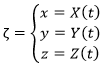
If we take two consecutive positions, ![]() and
and ![]() , the average speed is the vector carried by the rope
, the average speed is the vector carried by the rope ![]() The instantaneous speed on her side is a vector tangent to the trajectory.
The instantaneous speed on her side is a vector tangent to the trajectory.
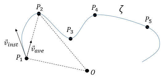
The direction of the speed vector defined thus the tangent to the trajectory. We can get rid of the length of the speed vector and keep its direction by dividing it by its intensity. As a result, we obtain a vector of length 1 tangent to the trajectory.
![]()
In the Cartesian system, it corresponds to
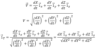
In this last expression, the time is not explicitly present. If we defined ds as the instantaneous displacement ![]() we can write
we can write
![]()
The length L of the trajectory is the sum of the lengths of the average displacements and, in the limit, to the integration of the lengths of the instantaneous displacements.
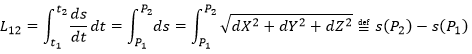
The length of the trajectory s is a parameter intrinsically related to the curve ζ as it doesn’t depend upon the choice of the origin point O, nor of the parameterisation of the curve ζ. It shows, in its infinitesimal version ds, the distance to make on the tangent of the trajectory.
The normal
The vector ![]() being defined, how do we express the geometric aspect related to the acceleration? By construction, the speed vector is tangent to the trajectory of the position vector. The acceleration vector is thus also tangent to the trajectory of the speed vector. How do we represent that in the space?
being defined, how do we express the geometric aspect related to the acceleration? By construction, the speed vector is tangent to the trajectory of the position vector. The acceleration vector is thus also tangent to the trajectory of the speed vector. How do we represent that in the space?
Let’s derivate the speed vector, giving explicitly its norm V and the direction ![]() :
:
![]()
The first term is proportional to ![]() and is thus parallel to the speed vector. The second term is necessarily perpendicular to it. Indeed, the trajectory of
and is thus parallel to the speed vector. The second term is necessarily perpendicular to it. Indeed, the trajectory of ![]() cannot be anywhere else than on a sphere because, by definition, its length does not change. As its derivative is tangent to this trajectory, it is thus tangent to the sphere and thus perpendicular to the radius of the sphere, i.e. to the vector
cannot be anywhere else than on a sphere because, by definition, its length does not change. As its derivative is tangent to this trajectory, it is thus tangent to the sphere and thus perpendicular to the radius of the sphere, i.e. to the vector ![]() .
.
We can define the normal vector ![]() as the derivative of the tangent vector.
as the derivative of the tangent vector.
![]()
λ is still to be determined.
- Algebraically
The acceleration ![]() is thus the sum of one tangent part
is thus the sum of one tangent part ![]() and one normal part
and one normal part ![]() , perpendicular to the first part.
, perpendicular to the first part.
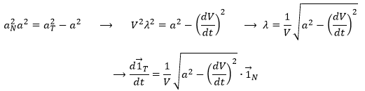
![]()
The length of the square of the acceleration is thus given by (the vector product of two perpendicular vectors gives zero)
![]()
And then
- Geometrically
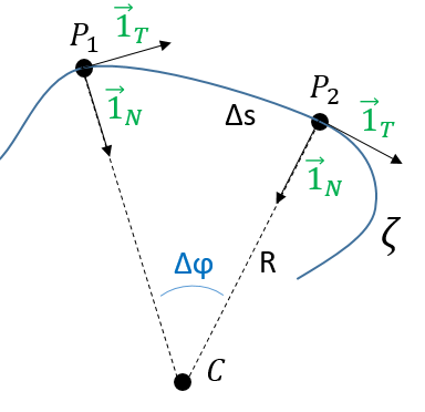
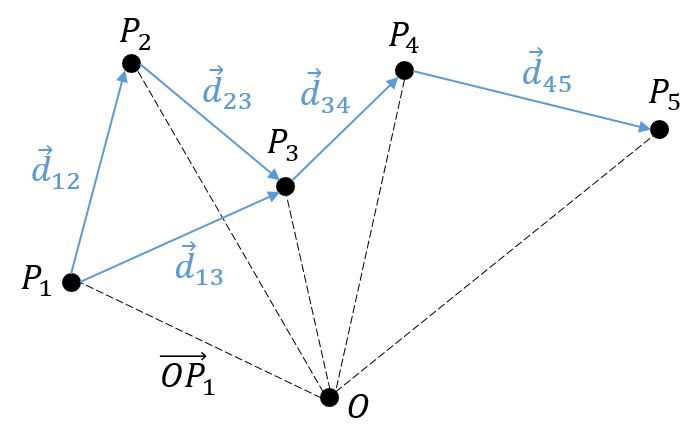
Given two consecutive positions of the point P on the trajectory ζ: ![]() and
and ![]() , and the direction of the speed
, and the direction of the speed ![]() and
and ![]() at the corresponding positions. The tangent unit vector
at the corresponding positions. The tangent unit vector ![]() , by definition, doesn’t change its length. However, its direction changes: it turns by an angle
, by definition, doesn’t change its length. However, its direction changes: it turns by an angle ![]() .
.
The two tangent vectors delimitate a plane P in which is also their variation ![]() . With these three vectors, we can build an isosceles triangle and thus evaluate the length of
. With these three vectors, we can build an isosceles triangle and thus evaluate the length of ![]() : 2 sin(
: 2 sin(![]() /2) and its angle with
/2) and its angle with ![]() : π/2-
: π/2-![]() /2.
/2.
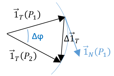
At the limit, when P2 tends towards P1, the length of ![]() becomes
becomes ![]() and the angle becomes thus π/2, i.e.
and the angle becomes thus π/2, i.e. ![]() becomes perpendicular to . As a result we can write
becomes perpendicular to . As a result we can write
![]()
λ corresponds thus to the angular speed of rotation of the tangent vector. To be more accurate, we see that if we extend the normal in P1 and in P2, they meet at the point C, and that this point C is, at the limit of ![]() , the centrum of the tangent circle of the curve ζ in P1 and P2. The angle
, the centrum of the tangent circle of the curve ζ in P1 and P2. The angle ![]() equals the length of the arc ∆s divided by the radius R of the circle. As a result,
equals the length of the arc ∆s divided by the radius R of the circle. As a result,
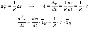
The radius R is called the curvature radius of the trajectory ζ at a given point. 1/R is called the curvature of ζ and the limit plane P formed by the tangent vector and the normal is called the osculating plane of the trajectory ζ.
The binormal
As the tangent ![]() and the normal
and the normal ![]() are defined, we can build a vector perpendicular to those two vectors: the binormal
are defined, we can build a vector perpendicular to those two vectors: the binormal ![]() . To do so, we make the vector product:
. To do so, we make the vector product:
![]()
This vector is perpendicular to the plane P of the trajectory and is oriented so that the three vectors ![]() can be overimposed to the three Cartesian vectors
can be overimposed to the three Cartesian vectors ![]() . Knowing the definitions of the speed and of the acceleration, we also can say that
. Knowing the definitions of the speed and of the acceleration, we also can say that
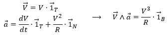
What allow us to determine the equation of the curvature radius R
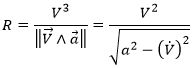
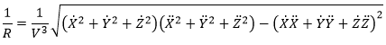
The dot over a variable means that it is its derivative over the time. Two dots will mean the second derivative, etc. The readability of the equation can be eased this way. In terms of components of the speed and of the acceleration, we have
Chapitre 4 : le mouvement, la vitesse et l’accélération
Il y a un mouvement si le vecteur ![]() change au fil du temps. On peut donc noter cette dépendance
change au fil du temps. On peut donc noter cette dépendance ![]() . La variation de la position est ce mouvement. En connaissant la position de l’objet P1, P2, P3, …à des moments consécutifs t1, t2, t3, … ,nous pouvons introduire le vecteur de déplacement
. La variation de la position est ce mouvement. En connaissant la position de l’objet P1, P2, P3, …à des moments consécutifs t1, t2, t3, … ,nous pouvons introduire le vecteur de déplacement ![]() comme le vecteur
comme le vecteur ![]() , et si l’objet continue à bouger,
, et si l’objet continue à bouger, ![]() , etc.
, etc.
Plusieurs observations peuvent être faites à ce stade:
- la position
 est l’ addition de la position précédente
  avec le déplacement
  .
.
![]()
- le déplacement
 est égale à la somme des déplacements et
  .
.
![]()
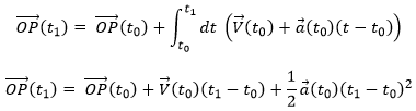
- cela peut sembler évident, mais il faut savoir que le nombre de positions est toujours plus que le nombre de déplacements. En conséquence, il est impossible de déterminer la position de l’objet à partir de ses seuls déplacements. Nous aurons besoin d’au moins une de ses positions.
Nous avons présenté ici l’opérateur d’addition + sur les vecteurs. Dans le système cartésien, il est facile de voir que les opérateurs d’addition et de soustraction sont simplement les opérateurs mathématiques + et – appliqués sur les nombres correspondant aux coordonnées.

La vitesse moyenne :
Maintenant que les déplacements sont définis, on peut considérer que le temps pour faire le déplacement entre P1 et P5 directement n’est pas le même que si on le fait avec des étapes intermédiaires. La vitesse moyenne est le déplacement moyen en unité de temps. Au temps t1, l’objet se trouvait en position P1 définit par le vecteur de position. Au temps t2, l’objet s’est déplacé à la position P2, définit par le vecteur de position. La vitesse moyenne entre ces deux positions est donc le déplacement de l’objet divisé par l’intervale de temps t2-t1.
![]()
La vitesse est dite moyenne car elle dépend des deux positions choisies. Une notation courante en mathématiques consiste à écrire les différences de deux valeurs par le signe Δ. Nous pouvons donc écrire
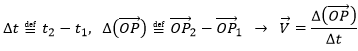
Que nous pouvons aussi écrire, avec la dépendance explicite sur le temps:
![]()
The instantaneous speed
One concept is now to get rid of the two positions to define an instantaneous speed, associated to a given position and a given time. To do so, we will bring the second point closer from the first and see what happens. We can’t only chose one point because the division by zero is not allowed. However, if this ratio continues to exist when the two points are almost identical, then the instantaneous speed is this value.
![]()
It is also the definition of the derivative of the position with regards to the time, calculated at t1. The limit towards zero of Δ will be noted d to obtain the notation corresponding to the usual derivative.
![]()
To indicate at which time we look for the speed, we use the notation
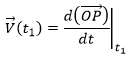
Each component of the speed is given by the derivative of the corresponding component of the position with regards to the time.
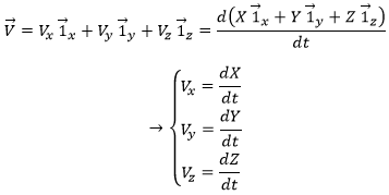
The acceleration
The same way we defined the speed as the variation of the position over time, the acceleration a is the variation of speed over time. We define an average acceleration as
![]()
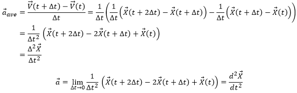
and the instantaneous acceleration as the derivative of the speed vector with regards to the time.
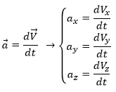
The acceleration can be obtained directly from the position by taking its second derivative. We introduce the notations
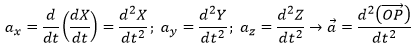
Note the difference of position of the square exponent: it is the derivative d/dt that is taken twice, not the object of the derivative. It is more evident if we use the definition of the derivative explicitly:
From acceleration to speed
As the acceleration is a difference of speed, there is thus always one acceleration less than there are speeds. From a speed at a time t1, on can determine the speed at a time t2 if we are given the acceleration during the interval of time.
![]()
From point to point, we can thus determine the speed:
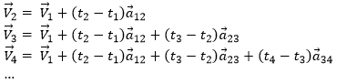
We can generalise this as
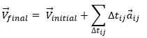
Obviously, the sum of the intervals of times equals the elapsed time:
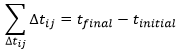
At the limit of the discrete time jumps, the sum becomes an integration
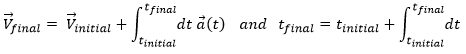
From the speed to the position
We can apply the same method on the speed to obtain the position:
Let insist on the physical meaning of this:
- the integration∫ is a sum,
- this sum is always made on a product,
- this product always contain an infinitesimal difference (here the time dt) and one finite quantity (here the speed V(t)),
- the sum ∫ is defined between a point of beginning and a point of end.
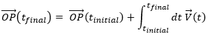
The uniform rectilinear motion
A uniform rectilinear motion (URM) is obtained when the speed of the object doesn’t depend upon time. The speed is thus constant and is defined at the initial time t0.
As the speed is constant, the acceleration is thus zero.
![]()
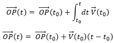
The equations for the position in each direction correspond to the equation of a straight line in the three dimensions space.
![]()
The uniformly accelerated rectilinear motion
Another simple problem is when the acceleration is constant. Similarly to the URM, here we easily find the speed:
![]()
And the position:
Chapitre 3 : le mouvement – la position
Le premier formalisme qui doit être connu en physique est le formalisme du mouvement. Un formalisme est associé à une certaine méthode mathématique rigoureuse, définissant des symboles et des règles qui sont communément acceptés, dans le but que tout le monde comprenne immédiatement le sujet discuté. Nous ne nous intéresserons pas à la prédiction du mouvement ni à sa cause, mais seulement à sa description.
Dans cette section, nous considérons que chaque objet peut être considéré comme un point sans volume.
La position :
Le mouvement est l’historique de la position d’un objet, la succession des positions de cet objet sur le temps. Pour définir la position de l’objet, nous avons besoin d’un système de référence dans lequel nous pouvons donner la position: coordonnées. Plusieurs systèmes de référence existent et il existe plusieurs façons de calculer les coordonnées des objets. Tous sont corrects mais certains sont plus pratiques que d’autres. Lors d’un voyage, vous ne donnerez pas votre position à l’égard du soleil, il en est de même en physique.
Plusieurs coordonnées sont généralement nécessaires pour déterminer la position exacte d’un objet. Si vous dites que vous êtes à 10 km de Paris, vous donnez une information sur votre position mais il nous manque au moins une coordonnée pour déterminer votre position. Habituellement, vous avez besoin d’une coordonnée par dimension du système.
Une dimension :
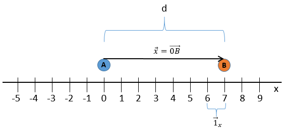
Nous choisissons une origine pour le système de coordonnées, le point zéro. Il est commode de choisir la position initiale de l’objet A comme origine mais ce n’est pas obligatoire. Ensuite, nous choisissons une direction qui sera les positions positives. Dans la direction opposée, nous avons les positions négatives. Toujours par commodité, les positions positives sont placées dans la direction vers laquelle nous devinons que l’objet se dirigera. Imaginez que l’objet se déplace vers un autre objet B placé à une distance d. Le vecteur de position indique la distance entre un objet et l’origine, et pointe vers l’objet avec une flèche. Le symbole des vecteurs est surmonté d’une flèche pointant vers la droite. Le vecteur de position pour B est
![]()
Où est le vecteur unité dans la direction x (la direction unique dans ce problème).
où ![]() est le vecteur unité dans la direction x (la direction unique dans ce problème).
est le vecteur unité dans la direction x (la direction unique dans ce problème).
 Deux dimensions :
La deuxième coordonnée est généralement orthogonale, perpendiculaire à la première coordonnée pour éviter un maximum de problèmes d’angle et pour bénéficier de la simplicité du calcul pour les triangles rectangles. Chaque coordonnée, a une direction. Le vecteur de position est maintenant défini par deux composants à partir desquels nous pouvons calculer sa longueur.
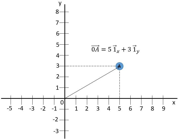
Le signe d’addition entre les deux vecteurs unitaires est comme ci-dessous et non comme l’addition de deux nombres usuels. Une autre façon d’écrire des coordonnées est de les mettre entre parenthèses. Si nous faisons cela, nous n’écrivons pas les vecteurs unitaires.
![]()
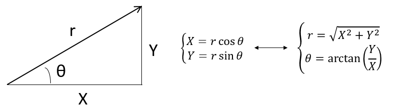
Ce système de référence, le système cartésien, n’est pas le seul qui puisse être utilisé (à deux dimensions pour déterminer la position d’un objet). Nous pouvons également positionner l’objet de sa distance r au point d’origine et un angle θ d’un axe. Ce système de référence est appelé le système polaire.
![]()
Il est possible de déterminer la relation entre les coordonnées X; Y dans le système cartésien et r; θ dans le système polaire en utilisant la relation définissant le cosinus, le sinus et la tangente:
Le vecteur d’unité ![]() peut ainsi être calculé.
peut ainsi être calculé.
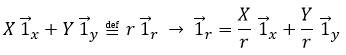
ou
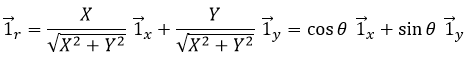
Nous pouvons également définir le vecteur de l’unité ![]() :
:
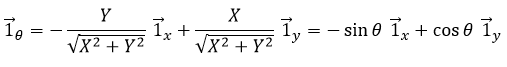
Les deux vecteurs d’unité polaire dépendent donc de θ qui doit donc être choisi consciencieusement.
Trois dimensions :
Une troisième coordonnée est ajoutée dans les systèmes de référence. Dans le système cartésien, nous ajoutons une coordonnée orthogonale aux deux précédentes
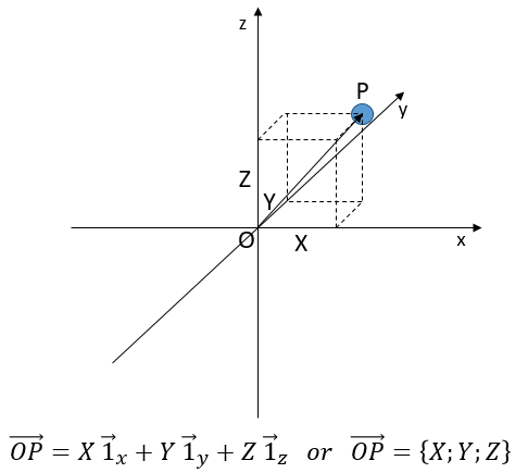
Dans le système polaire, nous avons besoin d’un second angle pour déterminer la position d’un objet. Nous prenons le premier de l’axe x dans le plan xy et le second angle est pris de l’axe z dans le plan zr de l’objet.
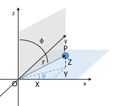
Encore une fois, le système cartésien peut être associé au système polaire.
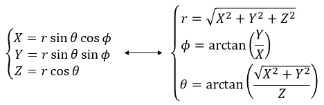
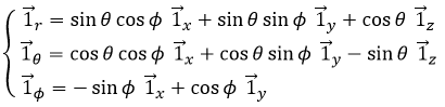
Les vecteurs unitaires sont définis comme :
Chapitre 10: cinétique chimique – réactions en solution
The big difference between a solution and a gas is the presence of a solvent. A viscous solvent means that there are more collisions between the molecules of reactant and the molecules of solvent, slowing down the molecules. The first obligation to obtain a reaction is that the reactants have to be close to each other. In a still solution, the species move by diffusion (if the solution is mixed manually or mechanically, the main transport process is called convection but the diffusion still acts with a minor influence). Once the reactants are nearby, they are caged in the solvent and remains nearby for a given time
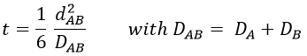
with DI the coefficient of diffusion of the species I. The reaction is the result of a vibrational movement. As for reactions of several steps, the global speed of a reaction will depend upon the slowest process. Diffusion can be the limiting factor.
Diffusion controlled reactions
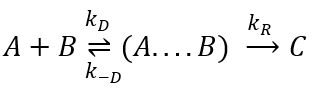
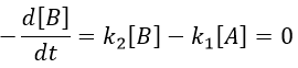
There are thus two steps in the reaction. The limiting step is the diffusion if k-D<<kR and the reaction is the limiting step if kR<<k-D. We use the assumption of stationarity for the concentration of the complex, i.e. the products C are formed at the same speed that the reactants are consumed.
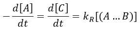
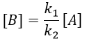
The concentration of the intermediate species is unknown but can be determined from the concentrations of the reactants if we know the constants of reaction.

We can now put this expression in the speed of reaction:
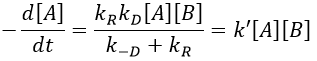
There are two limit cases:
- kR>>k-D: k’=kD, the reaction step is negligible in comparison to the time it takes to the reactants to meet. The reaction is limited by the diffusion.
- kR<<k-D: k’=kR.kD/k-D~kR, we can consider that the diffusion to approach or to go away from the other species is similar, so the speed of reaction is limited by the reaction itself.
Flow calculation
At the beginning of the experiment, i.e. t=0, the reactants A and B are uniformly distributed in the solution. No reaction took place yet and the solution is homogeneous. A short time after t=0, some reactants have formed products and a gradient of concentration can exist locally. The flow of diffusion J is given by the law of Fick:
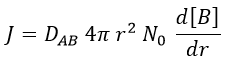
There is a flow of B towards A which is in the middle of a sphere or radius r. We integrate this expression from the smallest distance (dAB, i.e. the sum of the radii of A and B) to infinity.
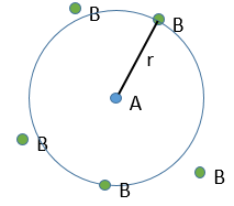
at r=dAB, [B]=0: the reaction is limited by the diffusion so we can consider that molecules of B that enter in contact with A react immediately. At an infinite distance r= ∞, the concentration of B is not affected by the presence of A and [B]∞=[B]0, the initial homogeneous concentration of B in the solution. Noting CB(r) the local concentration of B, the integration gives
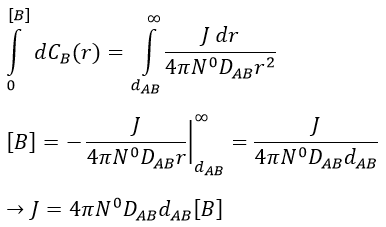
This value is the flow of molecules of B moving towards one molecule of A by unit of time. There are obviously more than one molecule of A in the solution.
At the stationary state,
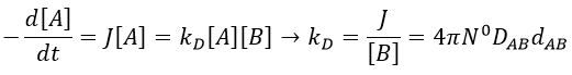
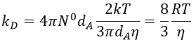
For instance, if we consider two usual molecules, dAB=0.6nm and DAB=2. 10-9 m2s-1, then kD~9.109mol-1ls-1. If the constant of reaction is of this order, then the reaction is limited by the diffusion. The constant is 20-100 times smaller in gaseous phases.
The equation of Stokes-Einstein connect the diffusion of a species with the viscosity of the solvent.
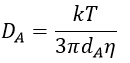
We can inject this expression in kD if A and B have similar dimensions to find that
In viscous solvents, if kD has this order of value, then the reaction is limited by the diffusion. A correction has to be considered if the species are charged:
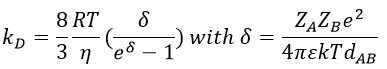
If the charges of A and B are opposite, then there is an attraction between the species and kD+->kD. If the charges are of same sign, then there is a repulsion and kD++<kD.
Speed of complex chemical reactions
The theories we have seen before are valid for elementary reactions only and approximations have to be done to study more complex reactions.
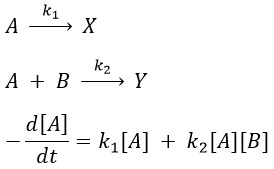
Parallel reactions
In this case several reactions of the same order (m=1 or 2) involve the same reactant.
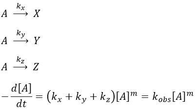
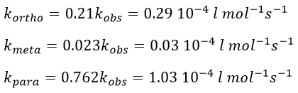
The experimental constant kobs is easily determined. The ratio of the concentrations of the products is equal to the ratio of the constants of reaction.
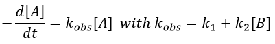
If there are two reactants, we put one of them in excess to obtain a pseudo order 1 reaction to determine the constant of reaction.
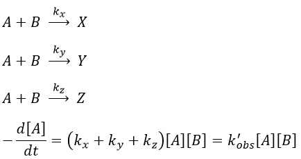
if [B]>>>[A] then k’obs[A][B]=k”obs[A] with k”obs=k’obs[A].
example: chloration of the tertiobutylbenzene
A chlorine atom can be added on tertiobutylbenzene on three different spots.
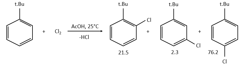
![]()
Knowing the global constant of reaction and the proportions of the three products, we can determine the constants of reaction of each reaction.
Parallel reaction with different orders
- with a single reactant
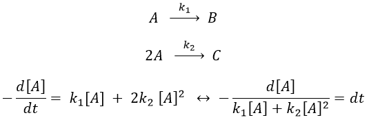
Luckily, mathematics give the solution for such an integral:
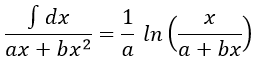
As a result,
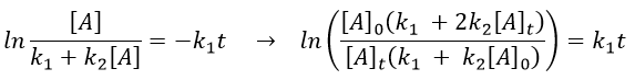
The relation is complex and the evolution of the concentration has to be studied through numerical programs. We can estimate the constants of speed with the method of initial speed.
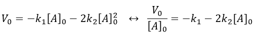
If we plot V0/[A]0 vs [A]0, we find an approximated value of k1 at the intersection of the ordinate with the curve and of k2 from the slope of the curve.
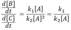
example of reaction: behaviour of the cis-trans- cycloocta 1,5-diene
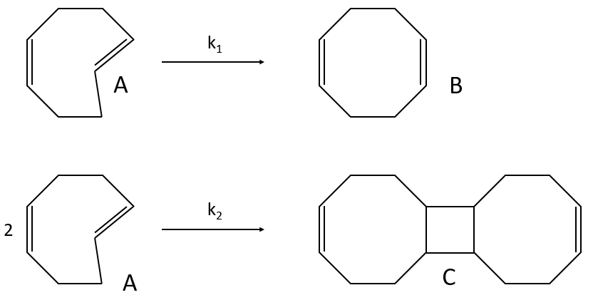
A difference with the case of parallel reactions of same order is that the ratio of the concentration of the product is not equal to the ratio of the constants of speed. If we measure the formation of the products, we find that the product B is produced faster and faster with regards to the product C:
Note that even if k2>k1, it means that the formation of B can be faster than the formation of C, immediately or at a given point of the reaction, as soon as the concentration of A is small enough. For instance, given an experiment with a concentration of A of 10-4mol/l, then k2 has to be 10000 times larger than k1 to obtain approximatively the same speed of formation for both products. As the reactions goes on, the speed of formation of C decreases furthermore.
Reaction involving a second reactant
We can simplify the problem with an excess of B so the second reaction becomes a pseudo-order 1 reaction.
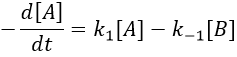
Reversible reactions of order 1
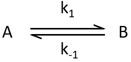
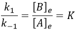
The constant of equilibrium K is the ratio of the concentration at the equilibrium of the products over the one of the reactants.

There is no notion of kinetics in this expression of the constant of equilibrium. But if we perturb the equilibrium, for instance by an abrupt modification of the temperature, the system has to adapt itself to the new conditions and the concentrations of the species varies.
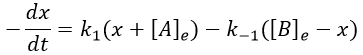
We can define x the deviation to the concentration of equilibrium (noted with a subscript e) such as
![]()
The evolution of x is independent of the current concentration and is given by
When the system reach its new equilibrium, the concentrations and x do not vary anymore.
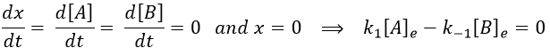
As a result, we obtain a new formulation of the constant of equilibrium of the reaction:
For a small perturbation of the equilibrium,
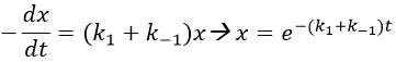
The transition between two equilibrium states is thus given by an exponential. If we plot the ln x versus the time, the slope of the curve gives the sum of the constants of speed k1+k-1. The characteristic time of relaxation tau to pass from one state of equilibrium at a temperature T to another one at T’ is
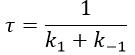
Knowing K and τ, we can find k1 and k-1.
Example: racemisation of two optically active enantiomers
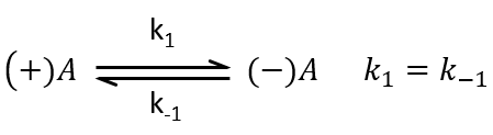
If we start from a solution with only one of the two enantiomers, there will be a spontaneous racemisation of the species in solution.
![]()
We can measure the variation of the angle of polarisation (optical activity α) of the solution over time.
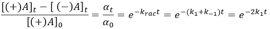
α tends towards zero because the optical activities of the enantiomers cancel each other. We see an activity when there is a overpopulation of one of the species.
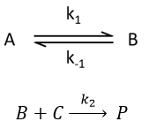
Consecutive reactions
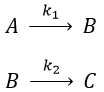
The concentrations of the three species can be followed.

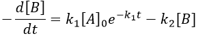
B is formed by the first reaction and is consumed by the second one, there is thus two components to the evolution of its concentration, one being positive and one being negative.
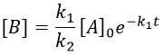
The first reaction is an order 1 reaction and the concentration of A is given by
![]()
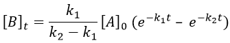
This expression can be injected in the expression for B.
It is a differential equation the solution of which is obtained by the sum of a general solution and of a particular expression. The solution is
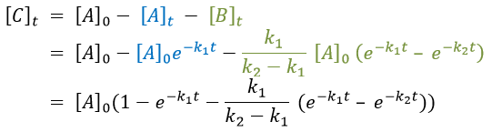
As the ratios between reactants and products is 1:1, the sum of the concentrations of the three species is equal to the concentration of A we put initially.
![]()
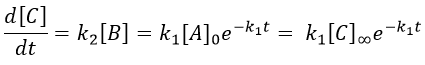
At any time, the concentration of the final product C is
After an infinite time, A and B are not in solution anymore and only the product C remain in solution.

The concentration of the intermediate product is highly dependent of the speeds of both reactions and shows a maximum at t=tBmax.
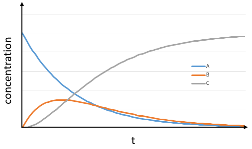
At t<tBmax, there is still plenty of reactant A that can form B. The concentration of B is not large enough to form quickly the final product C of the reaction. As a result, there is an accumulation of B. After tBmax, the rate of formation of B is smaller than its consumption.
If k2>>k1, then B is very reactive and does not accumulate. We can estimate that [B]t»0. If k2<<k1, then B is an intermediate with a long life time and that can accumulate up to a given concentration.
The concentration of C remains low during a period of induction and the evolution of C is not given by a simple function. We cannot obtain a simple kobs from its measurement. k1 can be measured from the concentration of A and k2 is found numerically from the expression of C or of tBmax.
Approximation of the stationary state
The previous case was still quite simple and involved only reactions of order 1. In more complex cases, we use the theorem of the stationary state. The hypothesis is that the concentration of the intermediate product is constant, i.e. it is consumed as fast as it is formed.
In the previous case, we would have obtained
It gives us the concentration of B as a function of [A]:
The expression for the concentration of A is known so
This expression, curiously dependant of the time for a species the concentration of which is considered as constant, can be inserted in the expression of C.
We can integrate this expression to obtain an expression of the concentration of C as a function of the time.

A is thus consumed in k1 and C is formed in k1 too. It is coherent with the fact that B disappears as soon as it is formed.
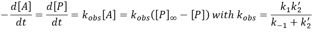
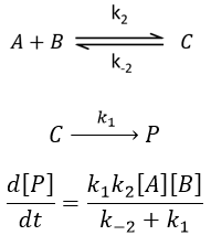
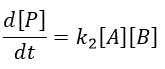
Reversible reaction of order 1 followed by a reaction of order 2
This case seems harder to solve.
Depending on the constants of speeds, several cases can be sorted:
- the equilibrium and the consumption of B have approximatively the same speed,
- the equilibrium is slow and B is consumed quickly,
- the equilibrium is quickly made with regards to the speed of the second reaction.
In a general way,
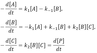
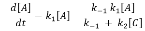
We make the assumption of a stationary state for B.

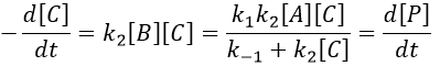
We insert this expression in the expression of A.
We still have two different concentrations that varies with the time in this expression ([A] and [C]). To obtain a solution, we need to find some limit conditions.
The final concentration of product P is either limited by the initial concentration of A or by the one of C, depending on which one is the smallest and which one is in excess. If we put C in excess, then
![]()
If [B] << [A]+[P], i.e. the case for which the hypothesis of stationarity is valid, then
![]()
and the expression can be simplified
If C was put in large excess, then we can consider its concentration as a constant and we find a pseudo order 1 reaction (k’2=k2[C]).
We can find the value of k1 if we use several different concentrations of C.
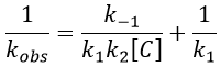
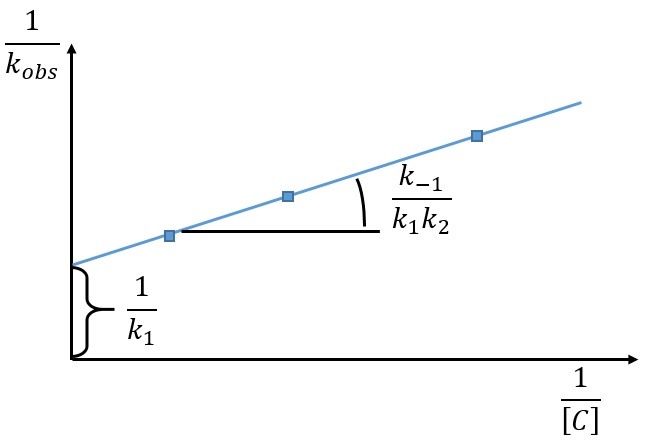
The intersection of the axis with the curve gives 1/k1 and the slope of the curve gives k-1/k1k2. However we don’t have the values of k-1 and k2.
There are two limit cases:
1) k2[C]>>k-1
B doesn’t turn back into A. The second step of the reaction doesn’t allow the first reaction to return to the equilibrium. As a result, both reactions can be considered as irreversible, what results in
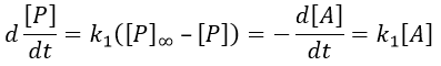
In this case, the order of the reaction is 1 even if C is not put in a large excess. [C] can be mathematically removed from the equation. The experimental constant of speed is equal to k1. The first step is thus the limiting step of the reaction.
Example: acetone + Cl2 in an acid middle
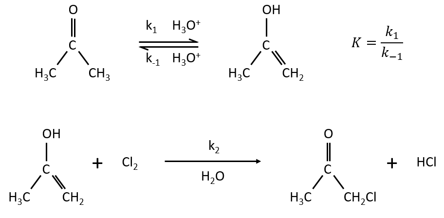
2) k2[C]<<k-1
The equilibrium of the first step of the reaction has the time to be reached. It leads to a global reaction of order 2.
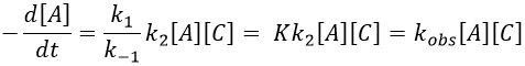
If C is in large excess, the reaction is of pseudo-order 1 as seen in the case 1, but if we put a very small concentration of Cl2 instead, then the expression for the speed changes:

Just by a modification of the experimental conditions, we can determine all of the constants of equilibrium of the enol-ketone tautomerism.
Reversible reaction of order 2 followed by an irreversible reaction of order 1
if k1>>k-2, then the first reaction has no time to return to the equilibrium and we can assume that the reactions are irreversible. The speed of the global reaction is limited by the first step of the reaction.
In the opposite case (k1<<k-2), we are still in the conditions of an apparent order 2 reaction but the constant of speed involves both reactions
Application: saponification of an ester
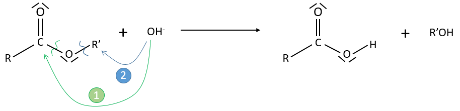
Experimental data tell that this reaction is of order 2 with the speed
![]()
However this expression still corresponds to two possible mechanisms. To determine which one is correct, we use an isotope of the oxygen (O 18) in the carbonyl group. The presence of the marked oxygen in the molecule indicates the good mechanism: during the reaction, this oxygen is equivalent to the one of the OH– group if the attack takes place on the carbonyl. Some marked oxygens can thus leave the molecule or change of position.
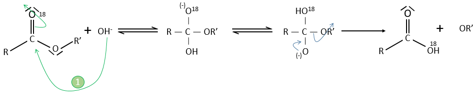
If R’O– is a good leaving group or not, we have two cases.
- Good leaving group
- Fast elimination, faster than the equilibrium
- The addition determines the speed
- V=k2[RCOOR’][OH–]
- Bad leaving group
- Equilibrium is established
- V=k1k2/k-2 [RCOOR’][OH–]
Chapitre 9: Cinétique chimique – Théories cinétiques
The following theories only apply to elementary reactions, i.e. in reactions in one step. The empirical relation of Arrhenius can be used (this relation is not limited to the elementary reactions):
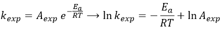
with kexp the kinetic constant found experimentally, Aexp the pre-exponential factor (same dimensions as kexp) and Ea the energy of activation. The goal is to measure experimentally Aexp and Ea. To do so, there are two theories in kinetics:
- the theory of the collisions and
- the theory of the state of transition.
Theory of collisions for bimolecular reactions (by W.C.Mc C.Lewis)
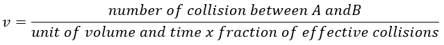
The principle is that all the collisions between molecules don’t lead to a reaction. There is a minimum of energy required to proceed. The speed of reaction can be characterised by
The speed of the molecules is not identical for each species. There is a distribution of speed, expressed by the distribution of Maxwell-Boltzman:
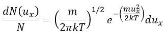
This expression gives the proportion of particles with the speed ux in the direction x. It gives a Gaussian centred at ux=0 because the particles can go in both directions of the axis. The surface under the Gaussian is constant but the curve becomes flatter if the temperature increases.
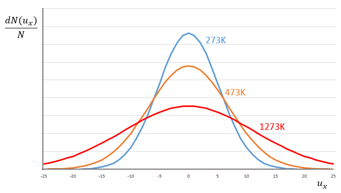
This change implies that more speeds are accessible to the particles if the temperature rises.
In 3 dimensions, the equation becomes
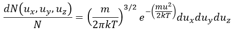
Now, instead of dux, duy and duz that apply to one direction of speed only, we want to get an element of volume in the phase of speed in all the directions. In the phase of speeds, it corresponds to a coquille of a sphere with a thickness du. The volume of the coquille is 4πu2du.
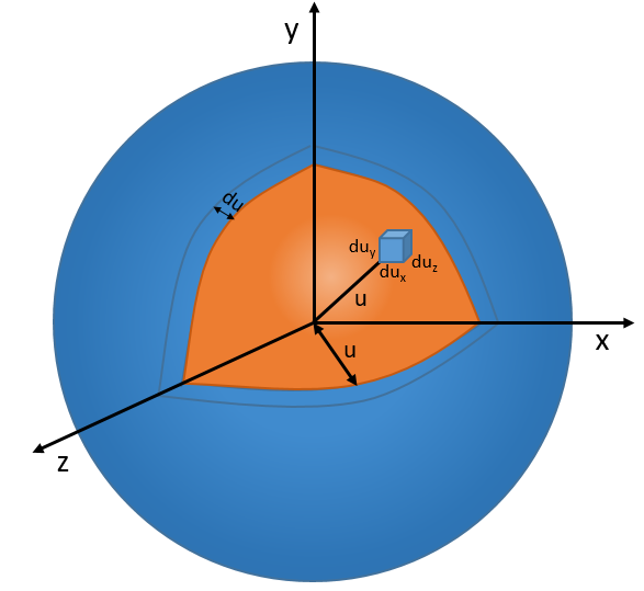
The equation of MB becomes
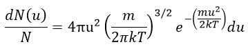
The consequence of the factor 4πu2 is that the curve is not a Gaussian anymore but a parabola and goes from u=0 to u= ∞ (the curve is symmetric for positive and negative values of u anyway).
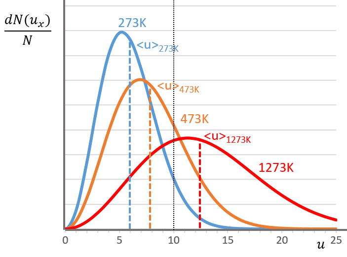
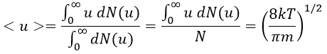
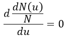
The maximum of the parabola is not at u=0 but it gives the most probable speed. Note that the most probable speed is not equal to the average speed <u>. Indeed, more than the half of the particles have a speed larger than the most probable speed. It is more and more displaced with larger temperatures.
The maximum of the curve can be found for
There is however a problem with this distribution of speed: if we strictly follow this distribution, the average speed of a gas such as N2 is approximatively 400ms-1, i.e. faster than the speed of the sound. If it was real, then when we open a bottle of a smelling volatile product (pyridine for example) at one side of the lab, we should instantly smell the odour of pyridine at the other side of the lab. It is not the case because we neglected the presence of other particles in the air. The collisions between the particles of the sample and the particles in the air reduce the spreading of the gas.
Model of collisions
There are two conditions for a reaction A + B à products to take place:
- there must be a collision between the reactants and
- the reactants must have an energy large enough to react.
The model relates the behaviour of one particle of A that moves straight forwards with an average speed <ur> through a static cloud of particles B without speed.
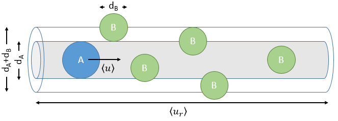
A and B are considered as solid spheres with a diameter dA and dB. The condition for a collision to take place in a period of time dt is that the centres of the spheres B are in the cylinder of length <ur>dt in the direction of propagation of A and diameter dA+dB centred on the A. The number of collision for one particle A by unit of time is given by
![]()
with NB the amount of particles B by unit of volume and rAB=dA+dB/2 the radius of the cylinder. There are several particles A moving simultaneously. The amount of collision is
![]()
There is one more thing that we have to consider: the particles B are also moving freely. Instead of the speed of the particle A, we will consider the relative speed of A with regards to B. Moreover, the angle of approach of the collision can vary. If we consider the collision between two identical particles, the collision can occur between two particles moving on the same line in opposite directions (angle=0°) with a speed <ur>=2<u>, between two particles moving almost alongside (angle ~180°) with a speed <ur>=0 or with angles between 0 and 180°.
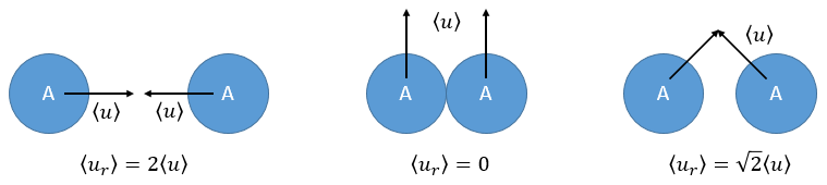
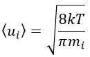
The average angle of collision is thus 90°. Considering this angle, the average speed for the collision between two identical particles is
![]()
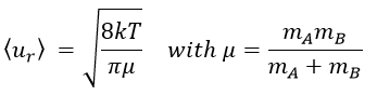
and for two different particles
![]()
The speed of a particle is given by the distribution of Boltzmann:
Inserting this expression in the previous one, we obtain
The amount of collisions by unit of time and volume is thus
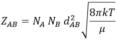
Note that if we count the amount of collisions between identical particles, we have to divide ZAA by 2 because otherwise we count each collision twice.
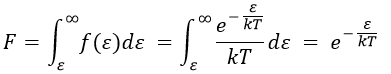
Now that we know the amount of collisions, we have to consider the fact that only a fraction F of them lead to a reaction between the particles. The particles must have an energy ε large enough to react and form products (ε > εmin). As for the speed, there is a distribution of kinetic energy f(ε) that gives the fraction of particles with an energy between ε and ε +dε.
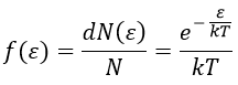
The distribution of energy depends on the temperature and also decreases if ε gets larger. The fraction of effective collisions contains all the collisions with molecules with an energy larger than ε, not limited to ε+dε.
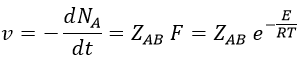
Macroscopically, the equation is
![]()
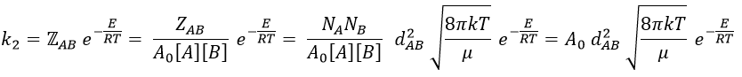
where A0 is the number of Avogadro. The speed of reaction is given by the frequency of collision multiplied by the fraction of effective collisions.
We define
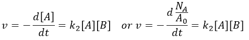
We know that we can write the speed of a reaction of order 2 as
The relation between the two expressions is thus that
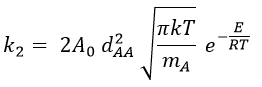
and for collisions between identical particles
Comparison between the results of the theory of collision with the empiric law of Arrhenius
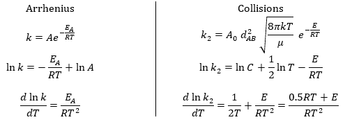
From this comparison we find that the experimental energy of activation EA is given by the energy required to have an effective collision plus ½ RT. If E>>>RT, then the energy of activation that is determined experimentally (i.e. from Arrhenius) is approximatively equal to E. As a result,
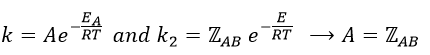
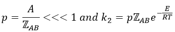
This match between the experimental observations and the theoretical values is only good for simple molecules. In the theory of collisions, we considered the particles as hard spheres. Otherwise, we introduce the factor of steric hindrance, or the factor of probability, p
Theory of the state of transition
This approach is more elaborated and can be applied to more complex molecules and to other phases than gases. This method takes the rotation and vibration into account.
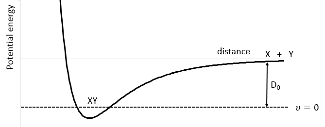
We know that there is a potential energy that is characteristic of a liaison. Starting from the vibrational level μ=0, i.e. the state where there is the highest probability to find the molecule, we need to give some energy to the liaison to break it and obtain a fragment X and Y.
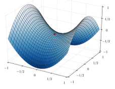
If a third molecule comes into play and is aligned with a diatomic molecule, there can be a collision introducing the third atom in the molecule and ejecting the atom at the opposite of the collision. To represent this phenomenon, we add one dimension to the figure above, leading to a surface of potential energy.
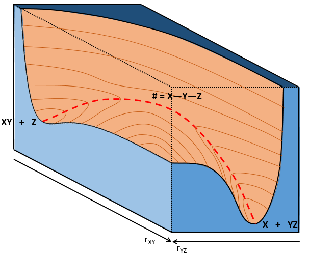
The path requiring the minimum energy is plotted in red and is called the reaction path and is the most probable path. Between the XY + Z and the X + YZ states, there is a state of transition # in which the liaison between Y and Z is not completely made and between X and Y not totally broken. The liaisons are extended and require more energy. Indeed, this state, called a complex of transition, is higher in energy than the state XY + Z and X + YZ. It is a saddle point in the space of reaction: a maximum in a direction and a minimum in another direction.
When the reaction reaches the transition state, the reaction can either go ahead or go back. The direction the reaction takes depends on the vibration and on the difference of energy between the states the reaction leads to. We can also represent the surface at two dimensions with isocurves of energy (see next figure).
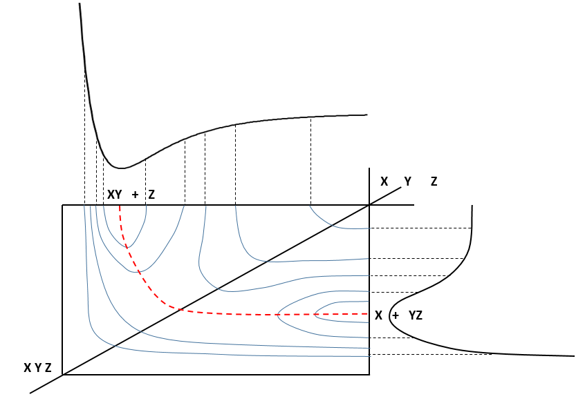
On the top side and on the right side of the graph, we see the potential curves of the liaisons YZ and XY respectively. The dotted line on the graph shows the path of lowest resistance. It is the most probable path of reaction. At the intersection between the axes, all three species are separated by the same, long distance and are not bound together. At the other side of the graph, there is no liaison between the atoms but they are very close to each other. If we plot the line connecting those two corners, the complex of transition is at the minimum of energy on this line.
If we plot the potential energy along the reaction path, we will obtain something like this:
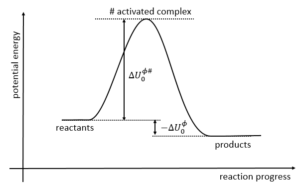
The ϕ symbol indicates that we are in normal conditions of temperature and pressure.
The model of the transition state
An equilibrium is considered to exist between the reactants and the complex of transition X#. From the complex of transition, products are formed with a frequency υt.
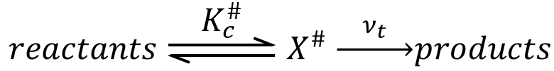
The speed of formation of the product is given by
![]()
Our problem is to determine the concentration of the complex of transition. We find it from the first step of the reaction. If this step is monomolecular (one reactant A), then
![]()
If the first step is bimolecular, then
![]()
If we replace υt Kc # by km, we find the experimental constant of reaction. To be perfectly correct,
![]()
where κ is the coefficient of transmission that is usually equal to 1.
Statistical formulation of km
There is a given number Q of states that are accessible to each molecule.
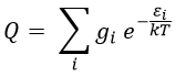
where gi is the degeneration of the state i and εi is the difference of energy between the state i and the ground state. The number of accessible states depends on the temperature.
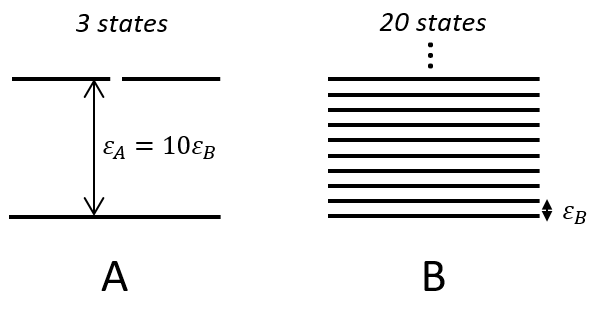
where ΔU0 is the difference of standard intern energy with regards to the zero point. We can also consider the molar standard intern energy but in this case we have to divide the functions of partition Q0(i) by A0V, A0 being the number of Avogadro.We can link the equilibrium constant of a reaction with the functions of partition of the molecules that take part in the reaction. Let’s consider a reaction
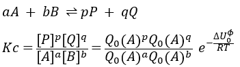
As km=υt Kc#, we can write
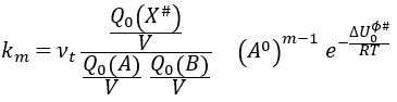
with m the order of the reaction. The function of partition of a molecule is related to its vibration, rotation and translation modes. For the complex of transition, the function of partition of the vibration mode can be isolated and is related to the frequency of vibration of the liaisons that are broken and made.
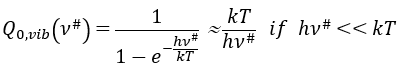
The function of partition is thus approximatively
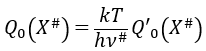
If the factor of frequency υt = υ#, then we obtain the statistical formulation of the constant of speed
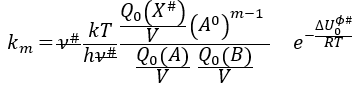
Q0(A) and Q0(B) can be determined by spectroscopy but Q0# has a life time too short to be correctly analysed (the time of a vibration, τ~100 femtoseconds). The functions of partitions depend on the temperature and we can globally write that
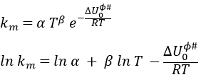
Taking the derivative of this expression with regards to the temperature, we obtain
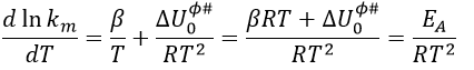
If we compare this expression to the law of Arrhenius, we have that
![]()
β is usually small so EA»ΔU0ϕ#.
Estimation of the pre-exponential factor of the equation of Arrhenius
We will consider the reactants as hard spheres.
![]()
In this condition, there is no vibration nor rotation to consider for them. They have thus only 3 freedom degrees. The function of partition of translation is
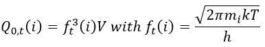
The transition complex is composed of two hard spheres and can thus rotate in two planes. We will assume that we can write the rotation and translation as two independent functions.
![]()
The mass we consider for the transition complex is simply equal to the sum of the mass of the two reactants: mAB#=mA+mB. The function for the rotation is
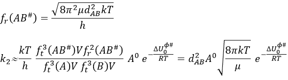
This expression for k2 is the same than the one obtain by the model of collisions but we obtained it with a totally different approach. As in the model of collisions, the molecules were considered as hard spheres and the model is not correct for more complex structures.
Thermodynamic formulation of km
In a gaseous phase, we have that
![]()
To obtain km in solutions, we have to divide Kc# by a power of the concentration cϕ=1mol/l
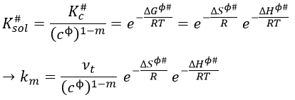
We want to connect this expression to the relation of Arrhenius. To do so, we need to make the approximation than υt=kT/h. As a result,
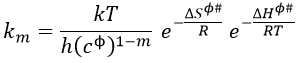
We will assume that ΔHϕ# and ΔSϕ# don’t depend upon T so that we can derivate the expression with regards to the temperature.
The enthalpy ΔHϕ# is related to the intern energy of activation ΔUϕ#. For ideal gases the relation is
![]()
Once the derivation d/dT is done, we obtain
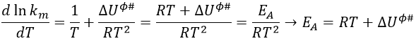
Previously in the theory of the transition state, we found EA= ΔU0ϕ#+βRT. Here β=1.
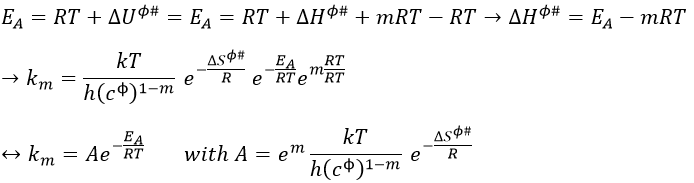
The variation of entropy is thus included in the pre-exponential factor. There is a variation of entropy during the formation of the complex of transition. For unimolecular reactions A → B in gaseous phase, the variation of entropy is approximatively equal to zero as there is no variation in the number of particles.
If the experimental pre-exponential factor is larger than 10-13s-1, it means that there is a variation of entropy during the process and that the reaction is a reaction of dissociation (A → B + C).
The fact that the variation of entropy is present in A is a big advantage with comparison to the model of collision where a steric factor was considered to obtain a result similar to the experimentations.
Femtochemistry
The femtochemistry allows to detect events with a timescale of the femtosecond. A. Zewail (Nobel prize in 1999 for his work on femtochemistry) studied in 1996 the transition states of chemical reaction with femtosecond spectroscopy. Using a rapid ultrafast laser technique (ultrashort laser flashes), the technique allows the description of reactions on very short time scales – short enough to analyse transition states in selected chemical reactions. For instance we can obtain 2 ethylene molecules from one cyclobutane and we want to determine the process. One possibility is the simultaneous cleavage of two liaison during one single vibration.
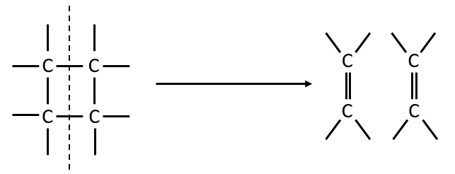
A second possibility involves the formation of a complex of transition wearing two radicals from the cleavage of one of the liaisons, and then the cleavage of the second liaison to obtain two ethylenes.
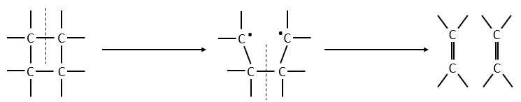
The second step of the reaction would be easier than the first step because the radicals help to the cleavage of the other liaison. The correct process is the one involving radicals. The life-time of the complex of transition is about 700fs and can be detected with femtosecond spectroscopy.
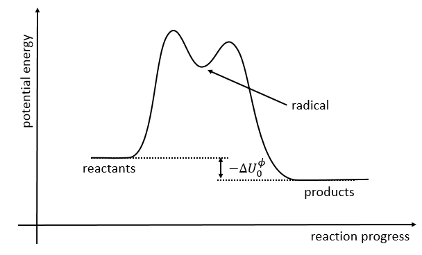
Application: photoreduction of the RuTAP by the GMP
We study here the transfer of one electron between the two species. The Ru(TAP)32+ (TAP= 1, 4, 5, 8-tetraazaphenanthrene) is a complex of coordination that can interact with DNA. We will next call it RuTAP.
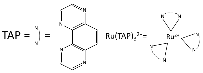
RuTAP absorbs in the visible (max at 420nm, orange-red).
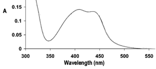
Instead of the analysis of the interaction of RuTAP with DNA, we replace the DNA by GMP (guanosine-5’-monophosphate) in this experiment. If we put RuTAP and GMP together in the dark, nothing happens. To observe a phenomenon, RuTAP has to be in an excited state. We illuminate the system at 420nm to excite RuTAP into RuTAP*.
![]()
The excited species will go back to its ground state through two possible reactions:
- the emission of a photon (not the same wavelength than the absorbed photon)
- the transfer of energy to the GMP. It leads to transitory products.
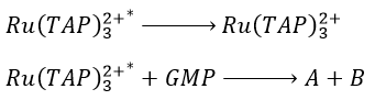
We want to determine the nature of A and B. We place the system in conditions such as the deexcitation through the emission of a photon does not occur. The illumination is only maintained during approximatively 10nanoseconds. However, the transfer of electron is completed over this period of time. After the pulse of light, we can study the evolution of the system through the emission of the solution. We don’t look at the wavelength in the range of the RuTAP (420nm) but in a range of frequencies where it does not emit: at 550nm, we find an intense signal that decreases quickly over time.
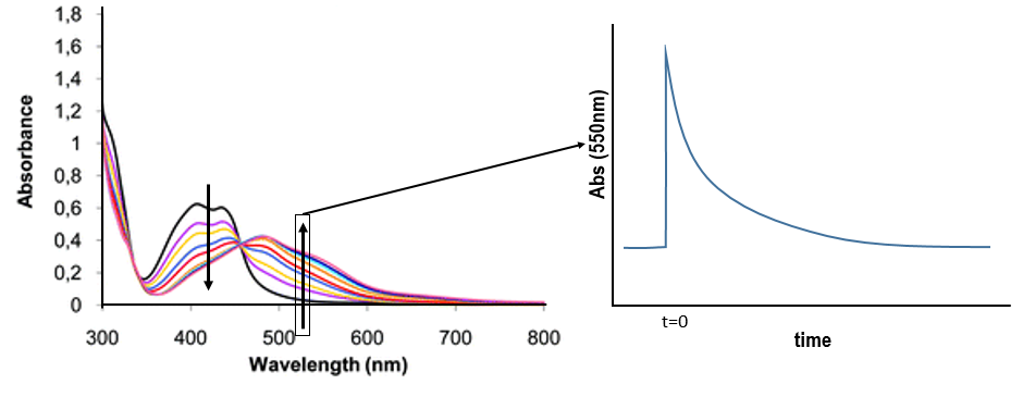
Before the pulse, nothing emits at 550nm. The formation of the emitting species is very fast but its decomposition is fast too. After the pulse, the transitory products of the reaction disappear over time and the signal comes back to zero. One hypothesis is that A is the reduced complex and that B is the oxidised GMP, respectively noted A=Ru1+ and B=GMP.+. This hypothesis is verified by a parallel experiment in which we measure the spectrum of Ru1+ alone.
We still meet one problem: the experiment was performed in a solution saturated in N2. When we repeat the experiment in presence of oxygen, the signal differs: the decrease of intensity is faster but the absorbance does not reach zero.
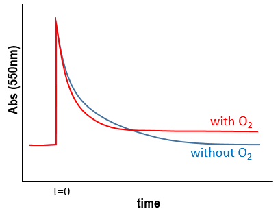
The oxygen generates an interference. To understand what happens, we analyse the signal in presence and in absence of oxygen. If we consider a monomolecular reaction, the decay should have the form of an exponential.
![]()
The characteristic time of this process is τ=1/k1. This type of decay is found in presence of oxygen (plus the fact that there is still a signal after the reaction).
If we consider a bimolecular reaction, with the same concentration for both reactants, then the decay is different.
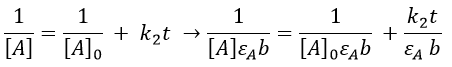
If we pose that k2’=k2/εAb, then

This decay is observed in absence of oxygen as expected for a reaction with two reactants
![]()
Note that we talk about equimolar reactants but the quantity of RuTAP and GMP that we put in solution at the beginning of the experiment does not matter. GMP.+ and Ru1+ are equimolar. The absorbance goes thus back to zero.
In presence of oxygen, there is a competition between the oxygen and the GMP.
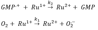
If the solution is saturated in oxygen (or if the system is open), then [O2]»constant and we find a pseudo order 1. This reaction occurs more than the reaction with GMP.+ because k1[O2]>>k2[GMP.+]. The signal does not go back to zero because some GMP.+ remains in solution (with a long life-time in comparison to the reaction). It is possible to determine the constants of speed k1 and k2 if we place ourselves in good conditions.
Chapitre 8: cinétique chimique – ordres de réaction
Kinetics is a field of the chemistry that studies the evolution of a chemical process over time. It gives practical information on the reaction and can help to determine its mechanisms. There is already two chapters discussing the basics of kinetics (1, 2) and we will now explore a bit deeper this field of chemistry. A chemical reaction can be written
![]()
Where A, B, C and D are chemical species and υI is the stoichiometric coefficient related to the species I. The reaction can be an elementary reaction or a complex reaction composed of several steps. The advancement of the reaction ζ can be followed by the variation of the amount of one species i.
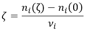
We can choose any species involved in the reaction as the studied species. The speed of reaction is given by the derivative of the advancement of the reaction at a given temperature. As we want only one characteristic speed of reaction, we divide the derivative by the stoichiometric coefficient of the studied species. Also note that products are formed while reactants are consumed. To have a positive speed, a minus sign is added if the studied species is a reactant.
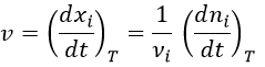
Instead of the amount of particles ni, their concentration is followed. Note that the volume is thus part of the equation but it is generally constant.
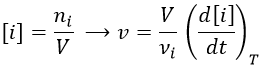
Instead of the concentration, we can use the partial pressure for gases.
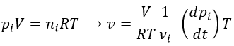
Experimentally, we will thus measure the concentration or the pressure of one species over the time. The concentration of a product increases over time while the concentration of a reactant decreases. The speed is defined positive and a minus sign must thus be placed before the derivative of the concentration of a reaction.
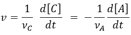
Yet, the speed of the reaction depends on the time: while approaching the end of the reaction, there is less reactant in the solution and the probability that the molecules of reactant are in contact so that they can react decreases. We want thus a measure that is independent of the time and characteristic of the reaction. On a graph of the concentration versus the time, the speed is proportional to plus or minus the slope of the curve. Obviously the slope changes over the time.
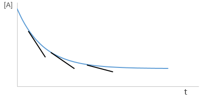
Reactions can be subdivided as a function of the order of reaction.
Reaction of first order
![]()
It is for instance a reaction of decomposition or a catalysed reaction. k1 is the constant of equilibrium, with 1 as index to suggest the order of reaction. A is one reactant and B is one product of the reaction. The instantaneous speed is directly proportional to the instantaneous concentration.
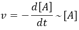
The coefficient of proportionality is the constant of speed k1.
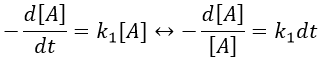
The units of k1 are s-1: when we look at the equation, [A] and d[A] have the same units –mol- and dt is in s. Each side of the equation has to have the same units so k1 is in s-1. The resolution of the equation is
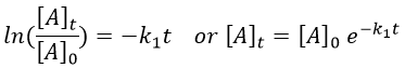
with [A]0 and [A]t respectively the initial concentration of the reactant and its concentration at time t. The concentration decreases exponentially over the time but we can plot the logarithm of the concentration ln[A] as a function of the time to find a straight line the slope of which is –k1.
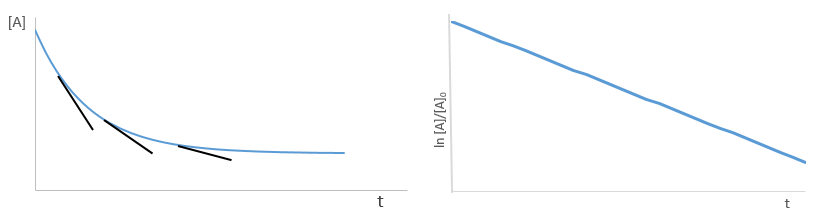
If instead of measuring the evolution of the concentration of the reactant we measure the evolution of the concentration of the product B, we know that both concentrations are related. The amount of B that is formed is equal to the consumed amount of A, i.e. the initial amount of A minus the amount of A that is still in solution. If there was no product is solution at the beginning of the reaction, then our final concentration of product will be the initial concentration of the reactant.
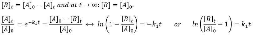
We can thus also find a straight line the slope of which is k1.
A time of half-life, i.e. the time required for the consumption of half of the reactant A, can be determined. It is not equal to the half of the time required to consume all the reactant.
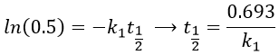
This time is independent of the initial concentration. After t1/2, the concentration of reactant is divided by 2. After 2 t1/2, the concentration is divided by 4. After 3 t1/2, by 8, etc. The measurement of those times we can confirm the value of k1 that was found by the slope of ln [A].
The concentration can be followed by a measure of the absorbance of the solution, of its pH, conductivity or optical activity.
Reaction of order 2
If we consider only one reactant and we don’t find the previous relations, the reaction can be of a higher order than the order 1. Two identical molecule can merge to form one new product, by condensation for example (amino acids).
![]()
In this case, the speed of reaction depends on the square of the concentration of the reactant.
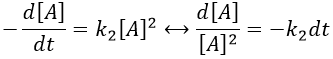
Note that this constant of reaction k2 has not the same units that the constant of reaction k1 of reactions of order 1. In d[A]/dt=k2[A]2, we have the square of a concentration at one side of the equation and a concentration at the other side (with a variation of time). The units of k2 are mol-1s-1. If we consider a gas, we will follow the pressure pA of the reactant.

As a result,

In a general way, we have kmp=kmc(RT)m-1 with m the order of the reaction.
The solution of the equation
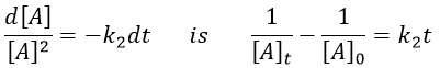
If we plot the logarithm of the concentration, we won’t find a straight line this time. To obtain one, we have to plot 1/[A]. The slope of the line is the constant of speed of the reaction.
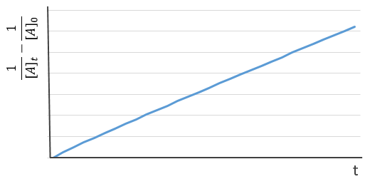
The half-life time is obtained from

This time, t1/2 depends on the initial concentration of the reactant. The half of the concentration is consumed over t1/2. The time to consume half of the remaining concentration [A]0’ (i.e. to consume the next [A]0/4) is not the same time but twice as long because the initial concentration is now [A]0’ and is the half of the initial concentration [A]0.
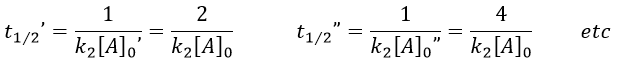
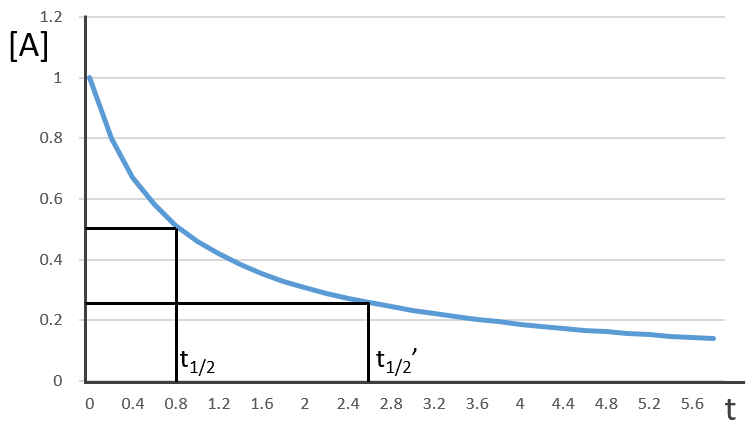
The half-life time becomes longer and longer with the advancement of the reaction.
Reactions of order 2 can also involve two different reactants.
![]()
A and B are consumed at the same rate but the concentrations can be different if there was an excess of one of the reactants.
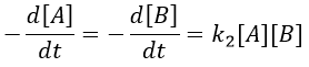
At a given time, a concentration x of A and of B has been consumed by the process. We can thus replace the concentration at that time by the difference between the initial concentration and x.
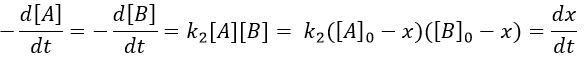
From two parameters we have now only one parameter, x and the equation can be solved.
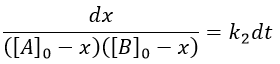
We can integrate the equation over the time of the reaction (from t=0 to t and from x=0 to x).
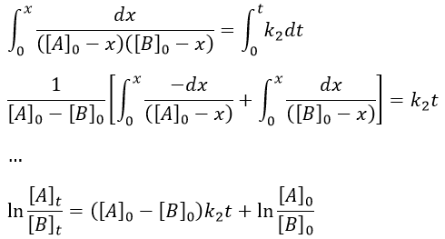
If [A]0=[B]0, then the ratio of concentrations [A]/[B] always remains constant but we won’t be able to determine k. The trick is to put one reactant in large excess and to follow the concentration of the second reactant. If one reactant is put in excess, then the expression for the concentration is more complicated. But if we put an excess large enough to consider the concentration of the other reactant as negligible, then
![]()
Then we obtain a pseudo-order 1 reaction.
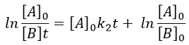
The second logarithm can be moved in the first:
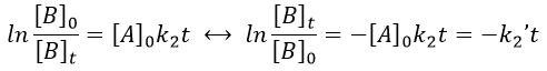
with k2’=[A]0k2 a kinetic constant of (pseudo)order 1. As we can find k2’, we know k2=k2’/[A]0.
The bimolecular nucleophile substitution (SN2) is a reaction the mechanism of which was found by regular kinetics studies.
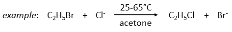
On the other hand the SN1 reaction showed extravagant results during the kinetics studies: the speed of the reaction was independent of the initial concentration of one reactant.
Reactions of order 0
In this kind of reaction, the speed of reaction does not depend on the concentration of one or more reactants.
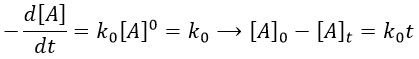
It is typically the case when the reaction is made through several steps. We also find order 0 if there is a limiting factor such as the surface of a catalyst. The speed of reaction is then constant over the time. If we take the case of one SN1, the reaction involves 2 reactants but does not show the expected order 2 for the reaction.
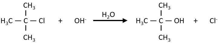
The reaction shows a kinetics of order 1 with regards to the chlorobutane and order 0 with regards to the hydroxide. The reason is that the reaction is made in two steps and the determining step is the first step in which OH– takes no part. The first step involves the formation of a carbocation from the chlorobutane, i.e. a reaction of order 1, and then a reaction of the second order that is much faster than the first reaction.
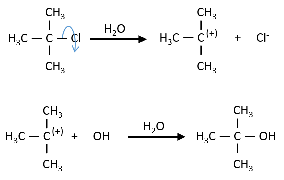
As the second reaction is much faster than the first, it is not this reaction that limits the global speed of reaction and we detect experimentally only the first reaction that does not include OH–. We can verify the order 0 by putting a large excess of the alkane in the solution and measure the evolution of OH–. It will decreases proportionally to the time and confirm the order 0.
An example of the utility of the kinetics is the synthesis of glycerol starting from epichlorohydrin made by Ernest Solvay.
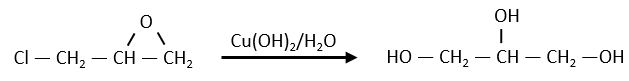
The glycerol and the epichlorohydrin are both transparent but once the reactant were put in the reacting tank and heated the system, the solution turned yellow-brown. They though that they overheated the system but it was still the same with a lower heating. A PhD in kinetics was consulted on the subject. He found out that the reaction is of order 0 with regards to the epichlorohydrin, meaning that the reaction involves several steps. If they heated up the reaction, they found an order 1 reaction. In fact, there is a determining step before the reaction: the dissolution of the epichlorohydrin into water.
As we have seen, a reaction can have a different order depending on the observed reactant. The global order n of the reaction is the sum of the orders with regards to each reactant.
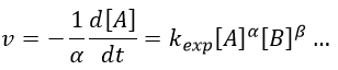
Where α, β, … are the order with regards to A, B, … and n=α+β+… is the order of reaction. There are several methods to determine experimentally the orders of a reaction with regards to the reactants
Method of integration
This method uses the relation between the evolution of the concentration of one given species over the time to determine the order of reaction with regards to this species: we verify if we can obtain a straight line on the graph of ln[A] vs time (order 1), of 1/[A] vs time (order 2) or of [A] vs time (order 0).
Method of half-life time fraction
We use here the properties of the half-life time if the reaction speed only depends on one of the reactants (the others are put in excess). We vary the initial concentration of the studied reactant.
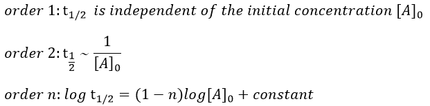
Method of isolement
All the reactants except one are in excess. We measure the order of the reaction with regards to this reactant.
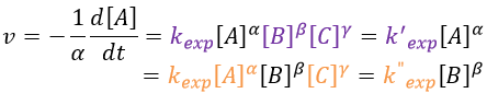
We proceed the same way with a different reactant (no excess of concentration) to determine the pseudo-orders of reaction with regards to each analysed reactant and we combine the result to find the order of reaction.
Method of the initial speeds
As usual we measure the evolution of the concentration as a function of the time. The tangent of the curve at t=0 gives the initial speed v0 (-v0 to be accurate). One reactant is not put in excess and is measured.
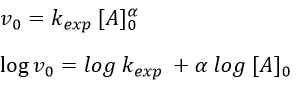
The experiment is repeated several times (it is quick because we only look at the beginning of the reaction) for several initial concentrations. This way we can determine kexp and α. This method is not very accurate because we measure a tangent at t=0.
When we study the kinetics of a reaction, we must always at least use the method of integration and of initial speeds and obtain concordant results. If it is not the case, the supposed mechanism is not correct.
Chapitre 7: chimie physique moléculaire – Degrés moléculaires de liberté: vibration et rotation
In the Born-Oppenheimer approximation, we froze the position of the nuclei to find the electronic energy. The position of the nuclei was considered as a parameter that can be modified and we were able to construct the Lenard-Jones potential for the liaisons or the surface (or hypersurface) of potential energy for molecules with more than one liaison. We will now discuss in further details about the vibration and rotation modes of molecules ant thus incorporate the movements of nuclei in the model.
The first step is to choose the set of coordinates in which we will work. A molecule with M nuclei has 3M coordinates: (xi,yi,zi) for each of the M atoms.
The laboratory axes system (LAS) is the first set of coordinates that we use. In this system we determine the position of the centre of mass of the molecule. Those 3 coordinates allow us to determine the translation of the molecule but not the rotation or the vibration modes: the centre of mass doesn’t move because of those modes.
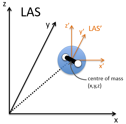
To determine those modes, we need two other sets of coordinates: the LAS’ that is fixed to the centre of mass of the molecule and consequently is independent of the translation and the MAS: molecular axes system that is fixed to the molecule and turns with it. 2 angles 0≤θ≤π and 0≤Φ≤2π are used to locate the linear molecules and a third one 0≤χ≤2π is needed for the nonlinear molecules. Those 3 angles are called the angles of Euler and are
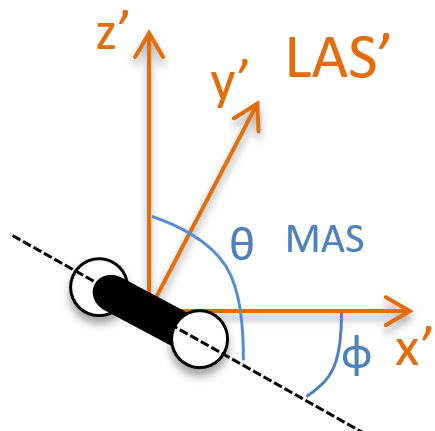
From the 3M coordinates, we used 5 (linear molecules) or 6 (non-linear molecules). The rest correspond to the modes of vibration of the molecule. In a diatomic molecule, there will be only one mode of vibration: M=2 and 5 coordinates are used to locate it.
To resume, the coordinates of one molecule are given by the vector
![]()
with 3M dimensions. The translation of the centre of mass is determined in the LAS
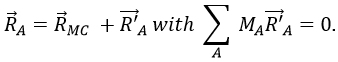
The condition here reflects the facts that the centre of mass does not move in the LAS’ referent. The MAS rotates with the molecule. To move into this referent, we apply the matrix S to the vector RA’.
![]()
The matrix S defines the orientation of the axes (x’,y’,z’) of the LAS’ from the coordinates (x,y,z) of the LAS:
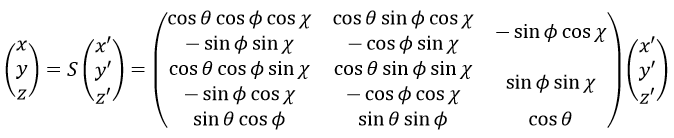
Small vibrations around the equilibrium RAeq are given by the vector dA
![]()
with the conditions of Eckart that
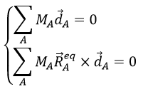
The first condition reflects that the centre of mass does not move because of the vibration and the second condition that there is no rotation in the MAS.
The kinetic energy of the molecule is in this notation
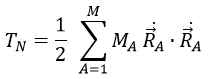
with MA the mass of the nucleus A and ṘA=dRA/dt. Replacing ṘA by its expression
![]()
We obtain (the red terms equal zero)
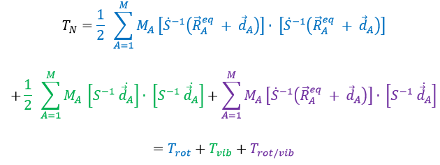
If Eckart is respected, then the interaction term Trot/vib can be neglected. We can thus approximate that the energies of rotation and of vibration are separable. The order of magnitude is indeed different: the vibration is found into the infrared while the rotation is observed in the microwave range.
![]()
Vibration
For a diatomic molecule, the oscillation is characterised by a force of recall
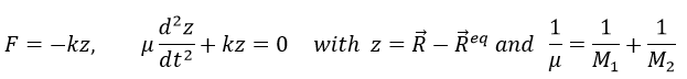
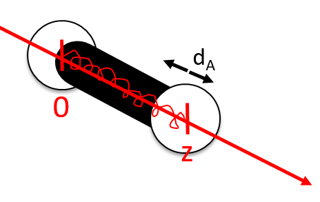
We find that
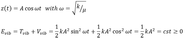
The energy of vibration can thus be approximated to a constant. The kinetic energy Tvib is always positive and is thus equal to
![]()
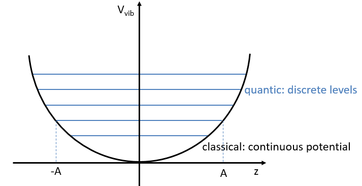
From the quantum mechanics, we know that
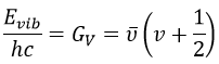
The separation in energy between the levels characterised by a number of nodes v=0, 1, 2, … There is thus regular a ΔGV=ῡ.
There is however a deviation to the harmonicity that we found. If we develop the potential as a series of Taylor, we obtain
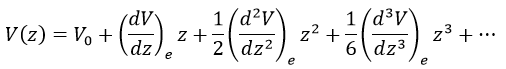
The two first terms are simply equal to zero (V0=0 and the potential is at a minimum at the equilibrium). The third term is the harmonic result that we just obtained but further terms express the deviation to the harmonicity. The potential of Morse gives an empiric formula that fits correctly the real potential.
![]()
The anharmonicity modifies slightly the energy of the states
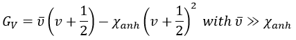
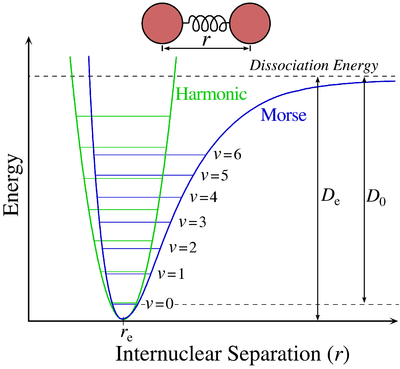
In the case of polyatomic molecules, we can consider that all the nuclei oscillate in phase, giving a base of 3M-6(5) independent movements. The result doesn’t noticeably differ from the diatomic molecule in this case.
Rotation
The rotation can be considered as a rigid rotation: the difference of frequency and of energy between the rotation and the vibrations is huge enough to make this approximation. The angular speed ω is thus identical for all the nuclei of the molecule.
![]()
The kinetic energy due to the rotation for a diatomic molecule is thus
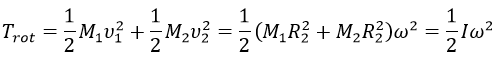
with I the moment of inertia that is common to the two atoms.
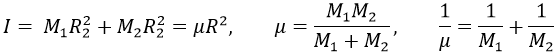
μ is the reduced mass of the molecule. The angular moment J is given by
![]()
Its absolute value is
![]()
For a diatomic molecule, we get
![]()
The angular moment and the kinetic energy are thus directly bound:
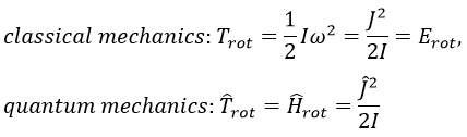
We can go from the classical mechanics to the quantum mechanics by the application of the Hamiltonian on a wave function.
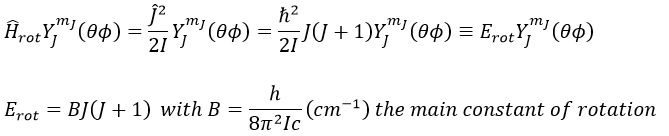
The multiplicity is gJ=2J+1. A small correction has to be added due to the centrifugal distortion, correction which is normally very small and negligible except when the rotation is very fast:
![]()
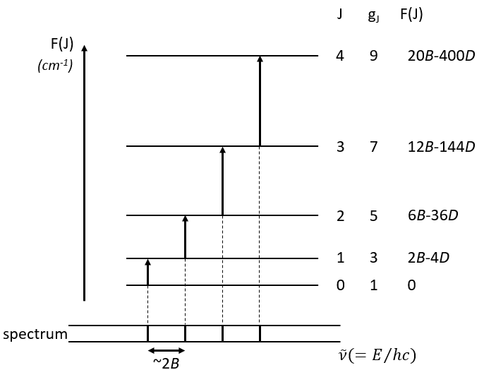
The spectrum of the rotation is thus composed of bands regularly spaced.
Chapitre 6 : chimie physique moléculaire – La théorie de la LCAO
This theory says that each molecular orbital Φa is described by a linear combination of atomic orbitals {χ} centred on the M nuclei of the molecule.
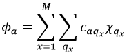
The molecular orbitals have the symmetry of one of the irreducible representations of the group G. This symmetry is taken into account in the LCAO coefficients. Some are null (some symmetries are not used) and some are equals in absolute value: only functions of same symmetry interact together to form molecular orbitals.
Given a MO Φa ∈ D(i) of G and the AO {χ}, we can adapt the atomic orbitals to the symmetry of D(i): {χ}à{χ(i)}. Then
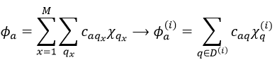
The advantage of doing this is that the number n(i) of functions χ(i) in the last expression is smaller than (or equal to) the number n of functions χ in the atomic orbitals. Let’s apply the LCAO theory to an example in which the orthonormal base is composed of two function {Ψ1, Ψ2}, i.e. a case where two states are in interaction with each other.
![]()
The secular determinant is
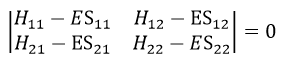
As the base is orthonormal, S is a delta of Dirac: S12=S21=0, S11=S22=1 and H12=H21. Posing that the two states H11 and H22 are equidistant from the zero energy, they are separated in energy by 2H:
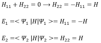
We can represent the problem as follow:
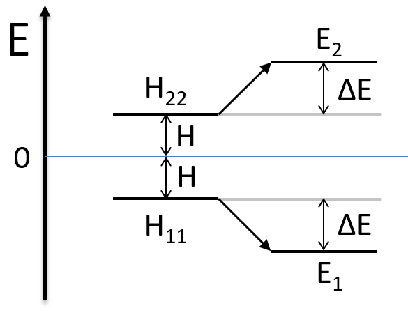
The secular determinant is thus reduced to
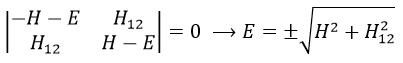
and
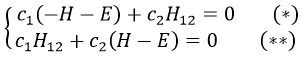
If we set c1=1, then c2=(H+E)/H12. The coefficients must still be normed.
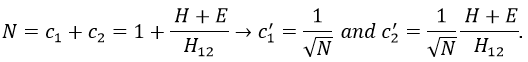
Two cases can be considered:
- H=0 with H12<0.
Two degenerated states interact with each other. The result of this interaction is that the states are repelling from each other. One is stabilised and the other one is destabilised by ΔE=H12. We will obtain a bonding state and an antibonding state. H12 is thus a measure of the interaction between the states. The bigger it is, the bigger is the separation between the resulting states. H was the distance between the states that interact together.
![]()
Posing that c1=1, then c2=-1. The coefficients must still be normed: c1=1/√2 and c2=-1/√2. As a result, the wave function of the state of energy E=-H12 is
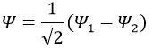
We can do the same for the second state (E=H12) and obtain
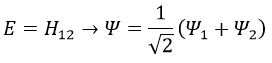
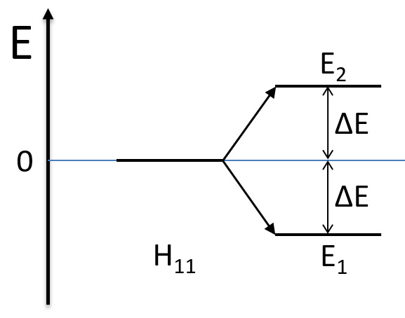
- H≠0 and H>>H12
The states that are interacting together have not the same energy. For instance, let’s consider H=2 and H12=-1/2.
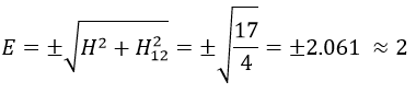
The interaction between the two states separated the states but just by a bit. The states did not mix a lot together.
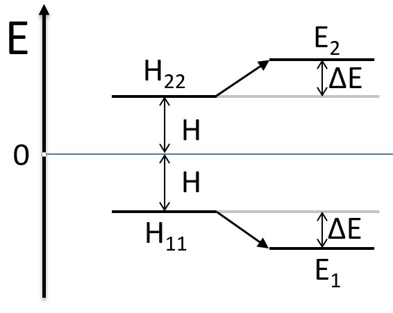
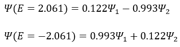
The mixing between two states is inversely proportional to the difference of energy between the states.
If H12=0, there is no interaction between the states. It is the case only when the states don’t share any symmetry, i.e. H12 can be different from zero only if Ψ1 and Ψ2 have common proper values with all the operators that commute with Ĥ. As a result, a triplet does not interact with a singlet even if the energies of those states are similar.
Rule of non-cancellation of an integral:
An integral is not equal to zero if the integrand is invariant with regards to all the operation of the group G, i.e. if the reduction of the direct product contains the totally symmetric irreducible representation D(1). In other words, the integral is different from zero if the integrand is totally symmetric.
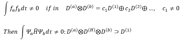
Cases of H2+ and H2
The orbitals 1s of the two atoms are interacting together to form molecular orbitals σg and σu. σg is a binding orbital resulting from a constructive interference:
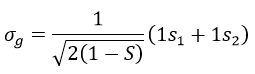
Here we considered that the base is not orthonormal. It is why the norm is 1/√(2(1-S)) and not 1/√2. S is the deviation to the orthonormal base
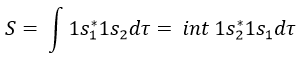
In an orthonormal base, S=0. The antibonding state σu is resulting from a destructive interference
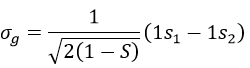
The interactions can be seen this way:
When the electron is in a molecular orbital such as the attraction it produces on both nuclei brings the nuclei closer to each other, the effect is binding.
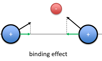
In the figure above, the electron is between the two nuclei. The attraction is produces on the nuclei is represented by the black arrows. The green arrows are the projection of the attraction on the axis passing by the two nuclei. The nuclei move thus in the direction of the other nucleus and remain thus together because of the presence of the electron.
If the position of the electron leads to a separation of the nuclei, then the effect is antibonding. The interaction of the electron-nucleus is positive but the intensities and directions are such as the nucleus-nucleus distance increases.
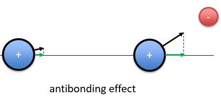
In the picture above, both nuclei are attracted by the electron but they move in the same direction with different speeds. The nucleus of the right moves faster than the nucleus of the left and the nuclei move thus away from each other.
The function 1s can be expressed as an exponentially decreasing function centred on the nucleus.
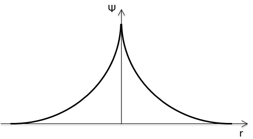
We can superimpose the functions 1s of two hydrogen atoms. In the case of σg, the functions add together:
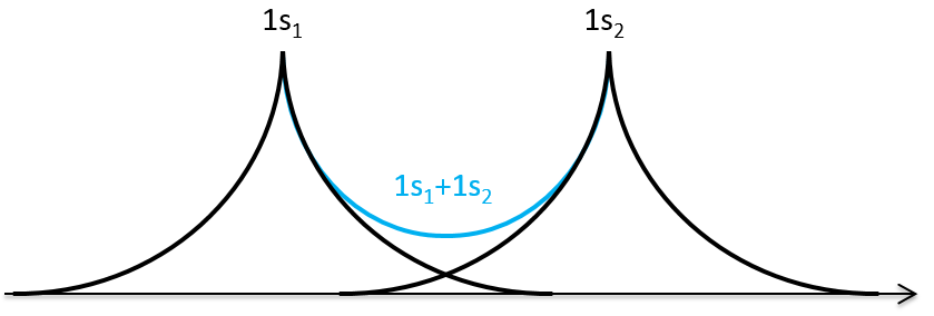
We can do the same for σu.
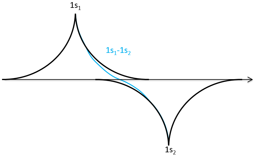
If we put those function to the square, we obtain the probability of presence of electrons.
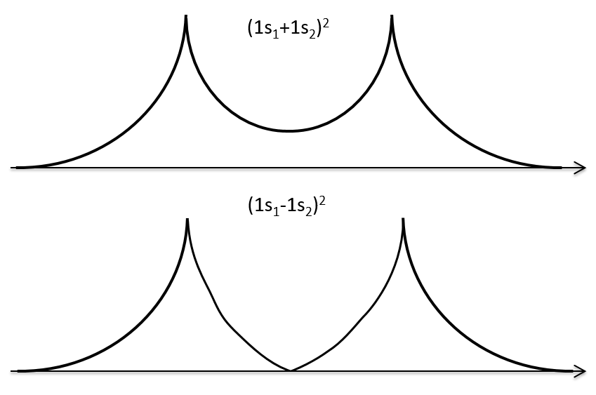
In the second case, there is a place between the nuclei where no electron can be found. No liaison can thus be done between the nuclei.
Interaction between 2p orbitals
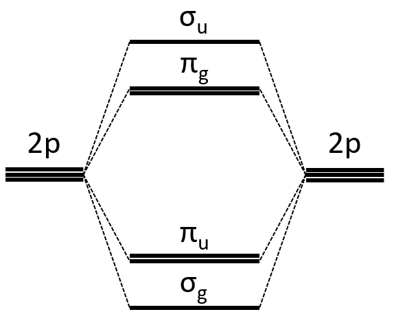
All the 2p orbitals don’t interact the same way. The 2pz orbitals interact together to give the σ orbitals. This time, it is not the sum of the atomic orbitals that give the molecular orbital of lower energy and the binding orbital σg.
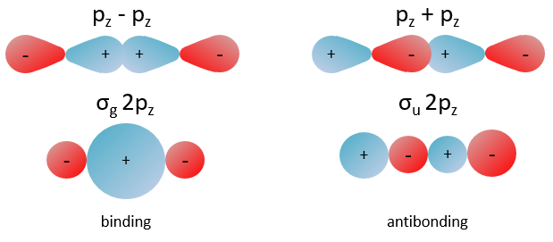
The other 2p orbitals (2px, 2py) lead to the π orbitals.
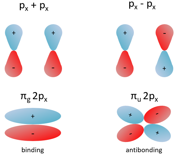
Note that the energy of the orbitals depends on the atoms. They all decrease in energy with Z but not with the same speed (see the figure below).
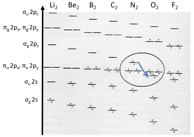
The energy of the πu orbitals is almost constant while σg 2px decreases quickly with Z. σg 2px falls under πu at O2.
The energy of the liaison between the two atoms increases up to N2 and decreases after because electrons are placed in antibonding orbitals.
The Walsh diagram
This diagram relates the energies of molecular orbitals of a molecule as a function of the angle that separates the liaisons. It helps to visualise the stability of the liaisons with regards to the symmetry of the molecular orbitals. The following figure shows the Walsh diagram for AH2.
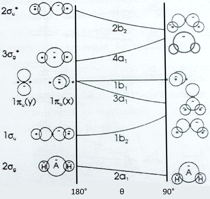
On the left one sees the linear molecules. As we go towards the right, the angle between the two liaisons goes towards the right angle, i.e. towards a bent conformation. As the bond angle is distorted, the energy for each of the orbitals can be followed along the lines, allowing a quick approximation of molecular energy as a function of conformation. As we move towards the top, the energy of the liaisons increases. Note that the 1πu orbitals are degenerated for an angle of 180° but separate if we change the conformation of the molecule.
For one molecule, we count the number of electrons of valence. For instance BeH2 has 6 electrons of valence (4 for Be and 1 for each H). We place 2 electrons by line, starting from the bottom (note that the 1a1 line, binding the σg orbitals, is not plotted. The last electrons are on the 1b2 line. One can see that the most stable angle for this molecule is 180°. For BH2 and CH2, the molecules are bent. If one electron is excited, then the conformation of the molecule can change.
Method of Hückel
This method limits the LCAO method to the π electrons. The reason is that a lot of physicochemical properties of the molecules can be explained by the π-π* orbitals. In the method of Hartree-Fock, the secular determinant was
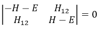
We have to solve the determinant for all the orbitals of the molecule, what can quickly become complicated. If we apply the method of Hückel on C2H4 for instance, there is only one π liaison in the molecule and thus only one secular determinant to solve. Considering two degenerated levels of energy α, the secular determinant is
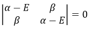
α=H11=H22 is the energy of the perpendicular to the plane atomic orbitals of the carbons and beta is the energy of resonance/interaction.
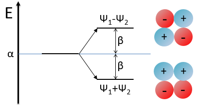
The solution found with this method (we won’t do it here) is close to the one obtained with the Hartree-Fock method that consider all of the electrons.
This method can be extended to other systems with π electrons if we pose that
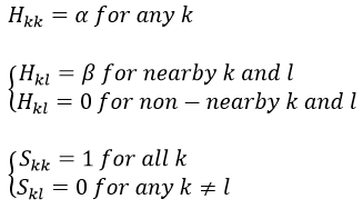
If we consider the butadiene, we consider it as the interaction of two π systems
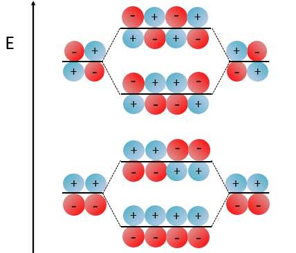
With the increase of π electrons, there are more binding states and one can see that, looking from the bottom to the top, the organisation of the orbitals follows a simple rule: the number of times that the signs are reversed increases by one at each orbital. One talk about the “wavenumber” of the orbitals. Indeed, on the lowest energy state, all the orbitals are aligned. There is no change of orientation of the orbital. On the second lowest state, the two orientations of the orbitals are present but they are grouped. There is only one change of orientation. The third level has 2 changes of orientations, there are 3 changes on the fourth lowest state, 4 on the fifth, etc… If we look at the orbitals as a wave, the wavenumber is indeed increasing with the energy of the state.
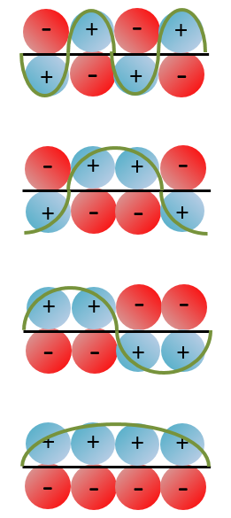
When the amount of π liaisons increases,
- the separation in energy between the states of same type (binding or antibonding) decreases and for a large amount of liaisons (in polymer for instance), we talk about a band of valence for the block of binding states and about a band of conduction for the block of antibonding states, separated by a gap.
- the amount of states increases in both bands,
- the separation in energy between the band of valence and of conduction decreases.
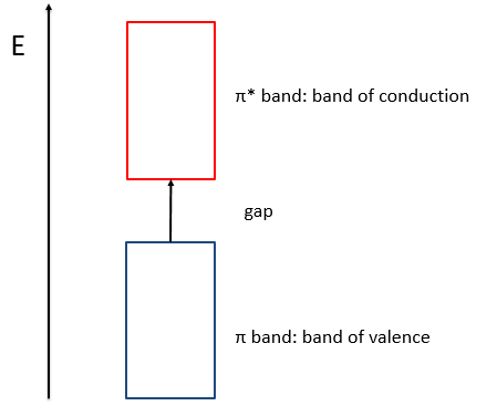
Chapitre 5: chimie physique moléculaire – Les méthodes d’approximation et la chimie quantique
We have seen quite a lot of new stuff up to now. We described monoelectronic and polyelectronic atoms and developed the description to molecules through the approximation of Born-Oppenheimer, the theory of groups and the CSOC. All of this teaches us how orbitals are and how they change during a reaction. Yet, we did not find the energies of the orbitals and can’t say which one is more stable than the others. The general equation is, as seen at the beginning of the course,
![]()
From the wave function we want to determine the energy of the orbitals but we can’t solve the equation exactly except for systems with one electron. For other species, we can only find an approached solution. To obtain it, we use the theory of perturbations or the method of variations.
Theory of perturbations
We can apply this theory to states that are independent of the time, i.e. stationary states. We can approximate the Hamiltonian and the energy of one state if this state is the result of a small perturbation λ of a state the solutions of which are known (Ĥ(0), E0).
![]()
The solutions are then expressed as a series of correction to the model at order zero.
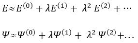
The corrections are calculated from the solutions at the order 0. For instance, the correction of order 1 are
![]()
The corrections usually decrease in intensity with their order but they will always approach the approximation from the exact solution. Note that we can go beneath the exact solution.
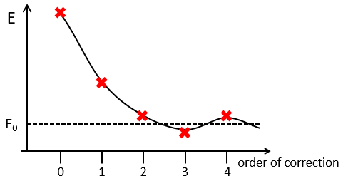
Method of variations
To find the exact energy, we use a trial wavefunction. This function has a known form but will probably not give the exact energy but will give us a superior born for the exact energy. Next, we modify the parameters of the trial wavefunction to obtain a better approximation of the energy. Unlike the method of perturbation, we can’t go beneath the exact energy with the method of variations. Each time we modify the parameters, we obtain a solution of lower energy and we approach the exact value of the energy. For instance if we chose a wavefunction with two parameters α and β. We can try to improve the values of the parameters to obtain the best possible approximation.
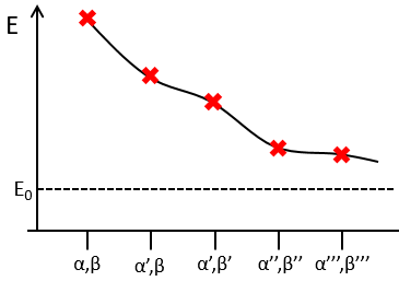
We reach an optimal estimation when the energy does not vary anymore when we change the parameters, i.e. when dE/dparameters=0.
Application to the helium
We will apply those two methods to estimate the energy of the helium. The exact solution is E=-2.903u.a. and the complete Hamiltonian is
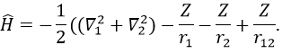
One model the solution of which is known is the hydrogenous model:
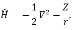
The solution of this model for 1 electron is
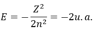
with Z the atomic mass and the quantic number n. As there are two electrons in the helium, we simply multiply the energy by 2 to obtain a first approximation from the hydrogenous model:
This approximation is far from the exact solution and overestimates the stability of the atom because we did not take the repulsion between electrons into account (the +1/r12 term).
The theory of the perturbation will start from this model and introduce the repulsion term as a pertubation of the model:
This estimation is way better than the hydrogenous model alone.
The method of variations is slightly different as we choose a wave function Ψ that depends on a few parameters that we may vary. As for the theory of perturbations, we select the hydrogenous wave function
As there are two electrons in the helium, we use a combination of two wave functions:
![]()
The parameter that we will vary is the effective charge Z=Zeff. One part of the charge of the nucleus is indeed hidden to one electron by the second electron.
From the chosen wave function, we find an equation for the energy that depends on Z
We optimise the parameter to obtain the best approximation that we can, such as dE/dZ=0. Solving this, we find
![]()
We apply this particular value of Z to the equation for the energy to find
![]()
This result is close to the exact solution.
Principle of linear variation: linear combination of atomic orbitals (LCAO)
In this method, we assume that Ж can be expressed as a linear combination of a base of functions {Ψ1, Ψ2, …}
where ci is the variational parameter associated to the wave function Ψi. These coefficients are adjusted to approximate the exact energy. For more simplicity, let’s take an example in which Ж is a linear combination of two wave functions Ψ1 and Ψ2.
![]()
It is corresponding to the case of H2:
![]()
The Hamiltonian is
![]()
Next we multiply this equation by Ψ1* and integer it over tau:
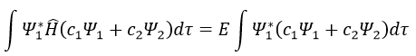
We can do the same with Ψ2*:
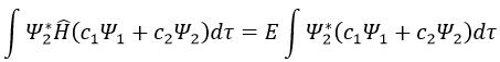
Now, we introduce Hij and Sij such as
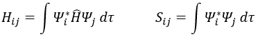
The previous integrals can be written
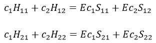
or
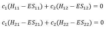
This system of two equations can be written as a 2×2 secular determinant
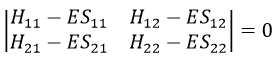
In a general way, it forms a n by n secular determinant if there are n wave functions (or particles)
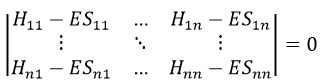
The n solutions of the secular determinant give the n most stable states of energy of the system. If we inject one of the energies E=Eq in the system, we obtain the optimised coefficients {ciq} related to the state q.
If the base is orthonormal, then
And then
If the base is complete, the linear combination corresponds to the exact solution due to the theorem of superposition (Quantum superposition is a fundamental principle of quantum mechanics. It states that, much like waves in classical physics, any two (or more) quantum states can be added together (« superposed ») and the result will be another valid quantum state; and conversely, that every quantum state can be represented as a sum of two or more other distinct states). The more the base is complete, the more one tends to the exact solution.
Method of Hartee-Fock
This method is an application of the variational method in which the trial wave function is a normalised determinant of Slater Ж = ∣ Φ 1 Φ 2 Φ 3… Φ N ∣. We try to minimise the energy of the orbitals (∂E/∂Φi=0) and to keep them orthonormal. We obtain a system of N coupled equations of Hartree-Fock that describe the movement of one electron in the averaged field ub created by the other electrons, such as
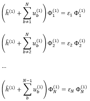
where εa is the HF energy of the molecular orbital Ψa. If we introduce the operator of Fock
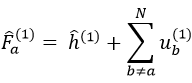
we can rewrite the system of N equations as
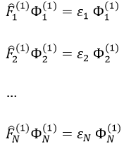
or on one line:
![]()
This equation only depends on the position and the movement of one electron, the effect of the other electrons being averaged. As the averaged field is determined by the orbitals that we are looking for, we have to solve the system of equations by iterations, starting from a set of orbitals of trial.
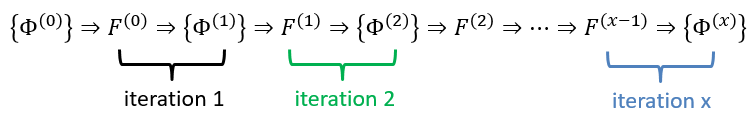
The convergence is guaranteed by the variational principle. In practice, we develop each orbital as a linear combination of Gaussian atomic orbitals centred on the nuclei. Then we iterate.