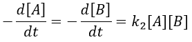
Chapter 10 : chemical kinetics – reactions in solution
The big difference between a solution and a gas is the presence of a solvent. A viscous solvent means that there are more collisions between the molecules of reactant and the molecules of solvent, slowing down the molecules. The first obligation to obtain a reaction is that the reactants have to be close to each other. In a still solution, the species move by diffusion (if the solution is mixed manually or mechanically, the main transport process is called convection but the diffusion still acts with a minor influence). Once the reactants are nearby, they are caged in the solvent and remains nearby for a given time
with DI the coefficient of diffusion of the species I. The reaction is the result of a vibrational movement. As for reactions of several steps, the global speed of a reaction will depend upon the slowest process. Diffusion can be the limiting factor.
Diffusion controlled reactions
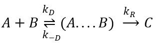
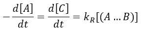
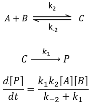
There are thus two steps in the reaction. The limiting step is the diffusion if k-D<<kR and the reaction is the limiting step if kR<<k-D. We use the assumption of stationarity for the concentration of the complex, i.e. the products C are formed at the same speed that the reactants are consumed.
The concentration of the intermediate species is unknown but can be determined from the concentrations of the reactants if we know the constants of reaction.

We can now put this expression in the speed of reaction:
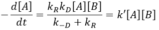
There are two limit cases:
- kR>>k-D: k’=kD, the reaction step is negligible in comparison to the time it takes to the reactants to meet. The reaction is limited by the diffusion.
- kR<<k-D: k’=kR.kD/k-D~kR, we can consider that the diffusion to approach or to go away from the other species is similar, so the speed of reaction is limited by the reaction itself.
Flow calculation
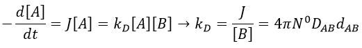
At the beginning of the experiment, i.e. t=0, the reactants A and B are uniformly distributed in the solution. No reaction took place yet and the solution is homogeneous. A short time after t=0, some reactants have formed products and a gradient of concentration can exist locally. The flow of diffusion J is given by the law of Fick:
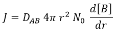
There is a flow of B towards A which is in the middle of a sphere or radius r. We integrate this expression from the smallest distance (dAB, i.e. the sum of the radii of A and B) to infinity.
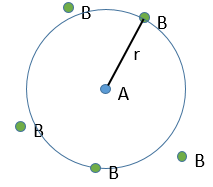
at r=dAB, [B]=0: the reaction is limited by the diffusion so we can consider that molecules of B that enter in contact with A react immediately. At an infinite distance r= ∞, the concentration of B is not affected by the presence of A and [B]∞=[B]0, the initial homogeneous concentration of B in the solution. Noting CB(r) the local concentration of B, the integration gives
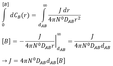
This value is the flow of molecules of B moving towards one molecule of A by unit of time. There are obviously more than one molecule of A in the solution.
At the stationary state,
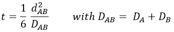
For instance, if we consider two usual molecules, dAB=0.6nm and DAB=2. 10-9 m2s-1, then kD~9.109mol-1ls-1. If the constant of reaction is of this order, then the reaction is limited by the diffusion. The constant is 20-100 times smaller in gaseous phases.
The equation of Stokes-Einstein connect the diffusion of a species with the viscosity of the solvent.
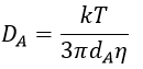
We can inject this expression in kD if A and B have similar dimensions to find that
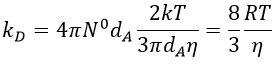
In viscous solvents, if kD has this order of value, then the reaction is limited by the diffusion. A correction has to be considered if the species are charged:
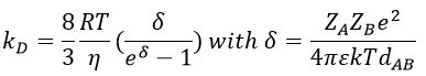
If the charges of A and B are opposite, then there is an attraction between the species and kD+->kD. If the charges are of same sign, then there is a repulsion and kD++<kD.
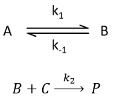
Speed of complex chemical reactions
The theories we have seen before are valid for elementary reactions only and approximations have to be done to study more complex reactions.
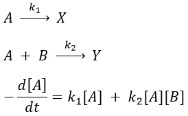
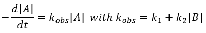
Parallel reactions
In this case several reactions of the same order (m=1 or 2) involve the same reactant.
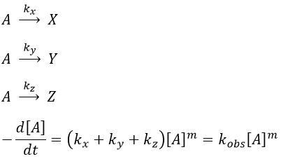
The experimental constant kobs is easily determined. The ratio of the concentrations of the products is equal to the ratio of the constants of reaction.
If there are two reactants, we put one of them in excess to obtain a pseudo order 1 reaction to determine the constant of reaction.
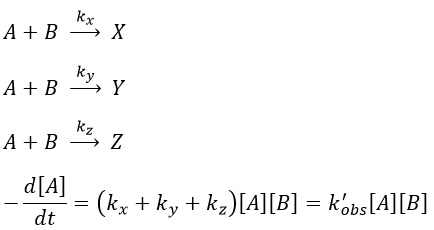
if [B]>>>[A] then k’obs[A][B]=k”obs[A] with k”obs=k’obs[A].
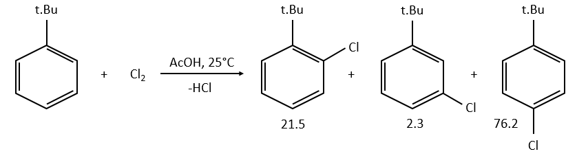
example: chloration of the tertiobutylbenzene
A chlorine atom can be added on tertiobutylbenzene on three different spots.
![]()
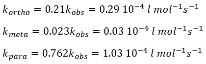
Knowing the global constant of reaction and the proportions of the three products, we can determine the constants of reaction of each reaction.
Parallel reaction with different orders
- with a single reactant
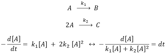
Luckily, mathematics give the solution for such an integral:
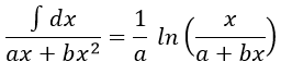
As a result,
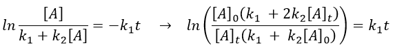
The relation is complex and the evolution of the concentration has to be studied through numerical programs. We can estimate the constants of speed with the method of initial speed.
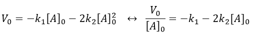
If we plot V0/[A]0 vs [A]0, we find an approximated value of k1 at the intersection of the ordinate with the curve and of k2 from the slope of the curve.
example of reaction: behaviour of the cis-trans- cycloocta 1,5-diene
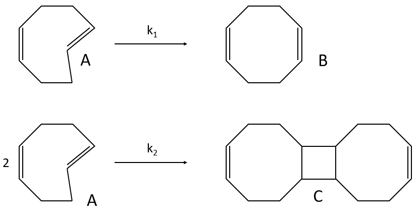
A difference with the case of parallel reactions of same order is that the ratio of the concentration of the product is not equal to the ratio of the constants of speed. If we measure the formation of the products, we find that the product B is produced faster and faster with regards to the product C:
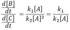
Note that even if k2>k1, it means that the formation of B can be faster than the formation of C, immediately or at a given point of the reaction, as soon as the concentration of A is small enough. For instance, given an experiment with a concentration of A of 10-4mol/l, then k2 has to be 10000 times larger than k1 to obtain approximatively the same speed of formation for both products. As the reactions goes on, the speed of formation of C decreases furthermore.
Reaction involving a second reactant
We can simplify the problem with an excess of B so the second reaction becomes a pseudo-order 1 reaction.
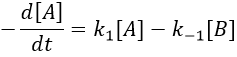
Reversible reactions of order 1
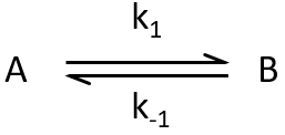
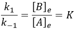
The constant of equilibrium K is the ratio of the concentration at the equilibrium of the products over the one of the reactants.

There is no notion of kinetics in this expression of the constant of equilibrium. But if we perturb the equilibrium, for instance by an abrupt modification of the temperature, the system has to adapt itself to the new conditions and the concentrations of the species varies.
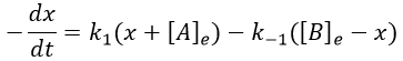
We can define x the deviation to the concentration of equilibrium (noted with a subscript e) such as
![]()
The evolution of x is independent of the current concentration and is given by
When the system reach its new equilibrium, the concentrations and x do not vary anymore.
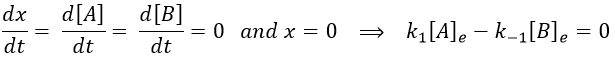
As a result, we obtain a new formulation of the constant of equilibrium of the reaction:
For a small perturbation of the equilibrium,
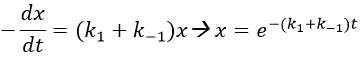
The transition between two equilibrium states is thus given by an exponential. If we plot the ln x versus the time, the slope of the curve gives the sum of the constants of speed k1+k-1. The characteristic time of relaxation tau to pass from one state of equilibrium at a temperature T to another one at T’ is
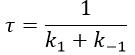
Knowing K and τ, we can find k1 and k-1.
Example: racemisation of two optically active enantiomers
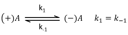
If we start from a solution with only one of the two enantiomers, there will be a spontaneous racemisation of the species in solution.
![]()
We can measure the variation of the angle of polarisation (optical activity α) of the solution over time.
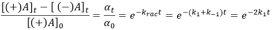
α tends towards zero because the optical activities of the enantiomers cancel each other. We see an activity when there is a overpopulation of one of the species.
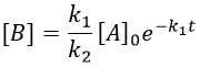
Consecutive reactions
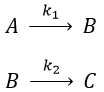
The concentrations of the three species can be followed.

B is formed by the first reaction and is consumed by the second one, there is thus two components to the evolution of its concentration, one being positive and one being negative.
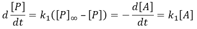
The first reaction is an order 1 reaction and the concentration of A is given by
![]()
This expression can be injected in the expression for B.
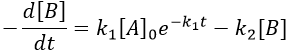
It is a differential equation the solution of which is obtained by the sum of a general solution and of a particular expression. The solution is
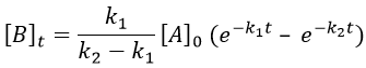
As the ratios between reactants and products is 1:1, the sum of the concentrations of the three species is equal to the concentration of A we put initially.
![]()
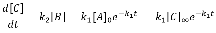
At any time, the concentration of the final product C is
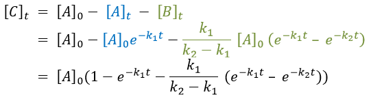
After an infinite time, A and B are not in solution anymore and only the product C remain in solution.

The concentration of the intermediate product is highly dependent of the speeds of both reactions and shows a maximum at t=tBmax.
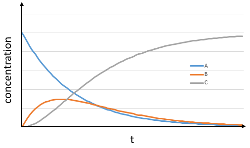
At t<tBmax, there is still plenty of reactant A that can form B. The concentration of B is not large enough to form quickly the final product C of the reaction. As a result, there is an accumulation of B. After tBmax, the rate of formation of B is smaller than its consumption.
If k2>>k1, then B is very reactive and does not accumulate. We can estimate that [B]t»0. If k2<<k1, then B is an intermediate with a long life time and that can accumulate up to a given concentration.
The concentration of C remains low during a period of induction and the evolution of C is not given by a simple function. We cannot obtain a simple kobs from its measurement. k1 can be measured from the concentration of A and k2 is found numerically from the expression of C or of tBmax.
Approximation of the stationary state
The previous case was still quite simple and involved only reactions of order 1. In more complex cases, we use the theorem of the stationary state. The hypothesis is that the concentration of the intermediate product is constant, i.e. it is consumed as fast as it is formed.
In the previous case, we would have obtained
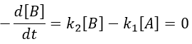
It gives us the concentration of B as a function of [A]:
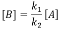
The expression for the concentration of A is known so
This expression, curiously dependant of the time for a species the concentration of which is considered as constant, can be inserted in the expression of C.
We can integrate this expression to obtain an expression of the concentration of C as a function of the time.

A is thus consumed in k1 and C is formed in k1 too. It is coherent with the fact that B disappears as soon as it is formed.
Reversible reaction of order 1 followed by a reaction of order 2
This case seems harder to solve.
Depending on the constants of speeds, several cases can be sorted:
- the equilibrium and the consumption of B have approximatively the same speed,
- the equilibrium is slow and B is consumed quickly,
- the equilibrium is quickly made with regards to the speed of the second reaction.
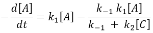
In a general way,
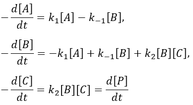
We make the assumption of a stationary state for B.

We insert this expression in the expression of A.
We still have two different concentrations that varies with the time in this expression ([A] and [C]). To obtain a solution, we need to find some limit conditions.
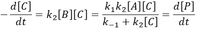
The final concentration of product P is either limited by the initial concentration of A or by the one of C, depending on which one is the smallest and which one is in excess. If we put C in excess, then
![]()
If [B] << [A]+[P], i.e. the case for which the hypothesis of stationarity is valid, then
![]()
and the expression can be simplified
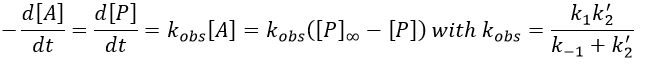
If C was put in large excess, then we can consider its concentration as a constant and we find a pseudo order 1 reaction (k’2=k2[C]).
We can find the value of k1 if we use several different concentrations of C.
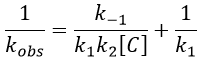
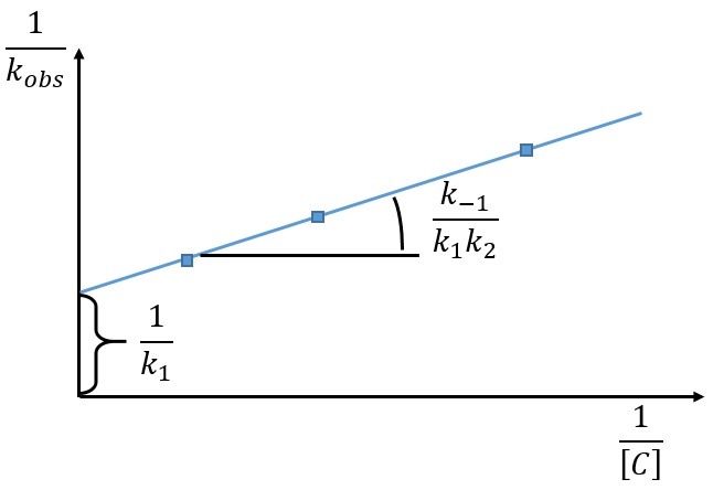
The intersection of the axis with the curve gives 1/k1 and the slope of the curve gives k-1/k1k2. However we don’t have the values of k-1 and k2.
There are two limit cases:
1) k2[C]>>k-1
B doesn’t turn back into A. The second step of the reaction doesn’t allow the first reaction to return to the equilibrium. As a result, both reactions can be considered as irreversible, what results in
In this case, the order of the reaction is 1 even if C is not put in a large excess. [C] can be mathematically removed from the equation. The experimental constant of speed is equal to k1. The first step is thus the limiting step of the reaction.
Example: acetone + Cl2 in an acid middle
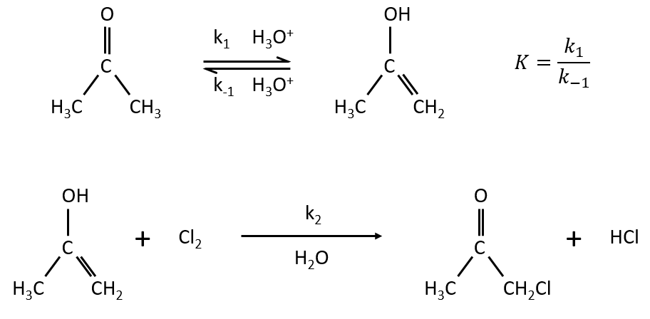
2) k2[C]<<k-1
The equilibrium of the first step of the reaction has the time to be reached. It leads to a global reaction of order 2.
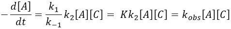
If C is in large excess, the reaction is of pseudo-order 1 as seen in the case 1, but if we put a very small concentration of Cl2 instead, then the expression for the speed changes:

Just by a modification of the experimental conditions, we can determine all of the constants of equilibrium of the enol-ketone tautomerism.
Reversible reaction of order 2 followed by an irreversible reaction of order 1
if k1>>k-2, then the first reaction has no time to return to the equilibrium and we can assume that the reactions are irreversible. The speed of the global reaction is limited by the first step of the reaction.
In the opposite case (k1<<k-2), we are still in the conditions of an apparent order 2 reaction but the constant of speed involves both reactions
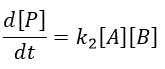
Application: saponification of an ester
Experimental data tell that this reaction is of order 2 with the speed
![]()
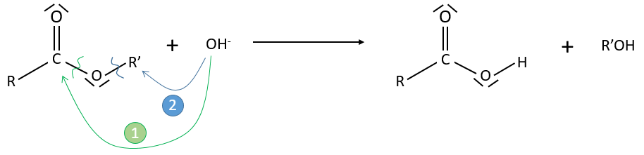
However this expression still corresponds to two possible mechanisms. To determine which one is correct, we use an isotope of the oxygen (O 18) in the carbonyl group. The presence of the marked oxygen in the molecule indicates the good mechanism: during the reaction, this oxygen is equivalent to the one of the OH– group if the attack takes place on the carbonyl. Some marked oxygens can thus leave the molecule or change of position.
If R’O– is a good leaving group or not, we have two cases.
- Good leaving group
- Fast elimination, faster than the equilibrium
- The addition determines the speed
- V=k2[RCOOR’][OH–]
- Bad leaving group
- Equilibrium is established
- V=k1k2/k-2 [RCOOR’][OH–]
Chapter 9 : chemical kinetics – kinetic theories
The following theories only apply to elementary reactions, i.e. in reactions in one step. The empirical relation of Arrhenius can be used (this relation is not limited to the elementary reactions):
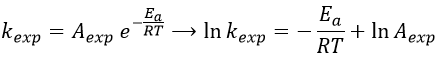
with kexp the kinetic constant found experimentally, Aexp the pre-exponential factor (same dimensions as kexp) and Ea the energy of activation. The goal is to measure experimentally Aexp and Ea. To do so, there are two theories in kinetics:
- the theory of the collisions and
- the theory of the state of transition.
Theory of collisions for bimolecular reactions (by W.C.Mc C.Lewis)
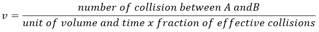
The principle is that all the collisions between molecules don’t lead to a reaction. There is a minimum of energy required to proceed. The speed of reaction can be characterised by
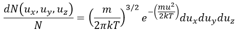
The speed of the molecules is not identical for each species. There is a distribution of speed, expressed by the distribution of Maxwell-Boltzman:
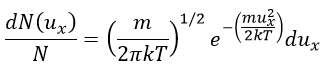
This expression gives the proportion of particles with the speed ux in the direction x. It gives a Gaussian centred at ux=0 because the particles can go in both directions of the axis. The surface under the Gaussian is constant but the curve becomes flatter if the temperature increases.
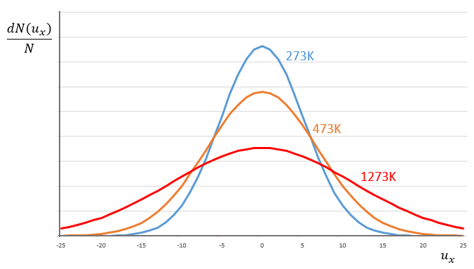
This change implies that more speeds are accessible to the particles if the temperature rises.
In 3 dimensions, the equation becomes
Now, instead of dux, duy and duz that apply to one direction of speed only, we want to get an element of volume in the phase of speed in all the directions. In the phase of speeds, it corresponds to a coquille of a sphere with a thickness du. The volume of the coquille is 4πu2du.
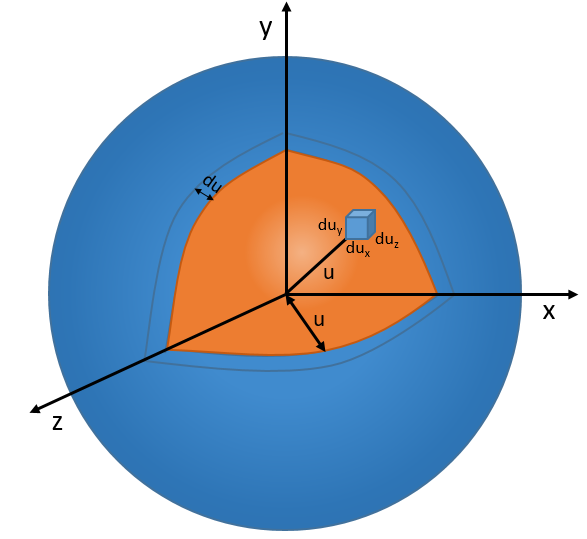
The equation of MB becomes
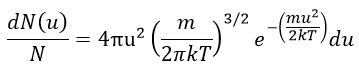
The consequence of the factor 4πu2 is that the curve is not a Gaussian anymore but a parabola and goes from u=0 to u= ∞ (the curve is symmetric for positive and negative values of u anyway).
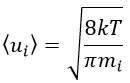
The maximum of the parabola is not at u=0 but it gives the most probable speed. Note that the most probable speed is not equal to the average speed <u>. Indeed, more than the half of the particles have a speed larger than the most probable speed. It is more and more displaced with larger temperatures.
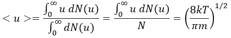
The maximum of the curve can be found for
There is however a problem with this distribution of speed: if we strictly follow this distribution, the average speed of a gas such as N2 is approximatively 400ms-1, i.e. faster than the speed of the sound. If it was real, then when we open a bottle of a smelling volatile product (pyridine for example) at one side of the lab, we should instantly smell the odour of pyridine at the other side of the lab. It is not the case because we neglected the presence of other particles in the air. The collisions between the particles of the sample and the particles in the air reduce the spreading of the gas.
Model of collisions
There are two conditions for a reaction A + B à products to take place:
- there must be a collision between the reactants and
- the reactants must have an energy large enough to react.
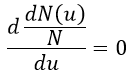
The model relates the behaviour of one particle of A that moves straight forwards with an average speed <ur> through a static cloud of particles B without speed.
A and B are considered as solid spheres with a diameter dA and dB. The condition for a collision to take place in a period of time dt is that the centres of the spheres B are in the cylinder of length <ur>dt in the direction of propagation of A and diameter dA+dB centred on the A. The number of collision for one particle A by unit of time is given by
![]()
with NB the amount of particles B by unit of volume and rAB=dA+dB/2 the radius of the cylinder. There are several particles A moving simultaneously. The amount of collision is
![]()
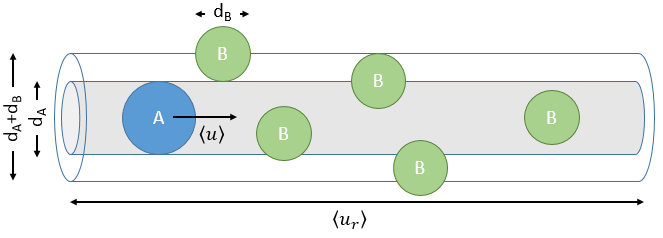
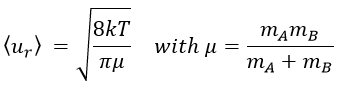
There is one more thing that we have to consider: the particles B are also moving freely. Instead of the speed of the particle A, we will consider the relative speed of A with regards to B. Moreover, the angle of approach of the collision can vary. If we consider the collision between two identical particles, the collision can occur between two particles moving on the same line in opposite directions (angle=0°) with a speed <ur>=2<u>, between two particles moving almost alongside (angle ~180°) with a speed <ur>=0 or with angles between 0 and 180°.
The average angle of collision is thus 90°. Considering this angle, the average speed for the collision between two identical particles is
![]()
and for two different particles
![]()
The speed of a particle is given by the distribution of Boltzmann:
Inserting this expression in the previous one, we obtain
The amount of collisions by unit of time and volume is thus
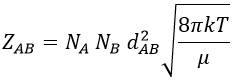
Note that if we count the amount of collisions between identical particles, we have to divide ZAA by 2 because otherwise we count each collision twice.
Now that we know the amount of collisions, we have to consider the fact that only a fraction F of them lead to a reaction between the particles. The particles must have an energy ε large enough to react and form products (ε > εmin). As for the speed, there is a distribution of kinetic energy f(ε) that gives the fraction of particles with an energy between ε and ε +dε.
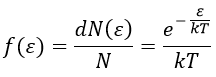
The distribution of energy depends on the temperature and also decreases if ε gets larger. The fraction of effective collisions contains all the collisions with molecules with an energy larger than ε, not limited to ε+dε.
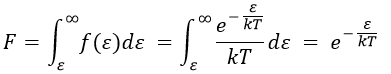
Macroscopically, the equation is
![]()
where A0 is the number of Avogadro. The speed of reaction is given by the frequency of collision multiplied by the fraction of effective collisions.
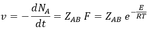
We define
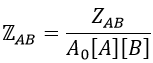
We know that we can write the speed of a reaction of order 2 as
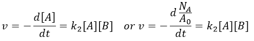
The relation between the two expressions is thus that
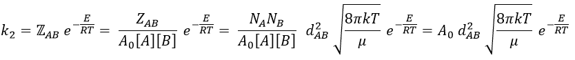
and for collisions between identical particles
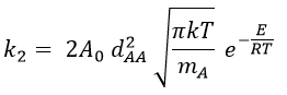
Comparison between the results of the theory of collision with the empiric law of Arrhenius
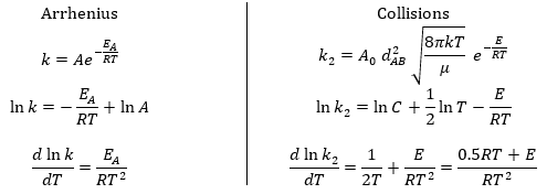
From this comparison we find that the experimental energy of activation EA is given by the energy required to have an effective collision plus ½ RT. If E>>>RT, then the energy of activation that is determined experimentally (i.e. from Arrhenius) is approximatively equal to E. As a result,
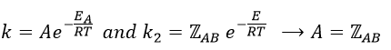
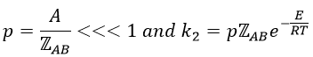
This match between the experimental observations and the theoretical values is only good for simple molecules. In the theory of collisions, we considered the particles as hard spheres. Otherwise, we introduce the factor of steric hindrance, or the factor of probability, p
Theory of the state of transition
This approach is more elaborated and can be applied to more complex molecules and to other phases than gases. This method takes the rotation and vibration into account.
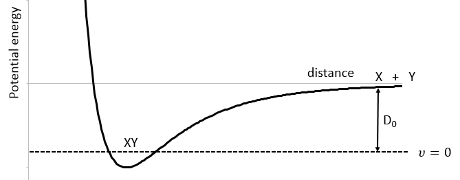
We know that there is a potential energy that is characteristic of a liaison. Starting from the vibrational level μ=0, i.e. the state where there is the highest probability to find the molecule, we need to give some energy to the liaison to break it and obtain a fragment X and Y.
If a third molecule comes into play and is aligned with a diatomic molecule, there can be a collision introducing the third atom in the molecule and ejecting the atom at the opposite of the collision. To represent this phenomenon, we add one dimension to the figure above, leading to a surface of potential energy.
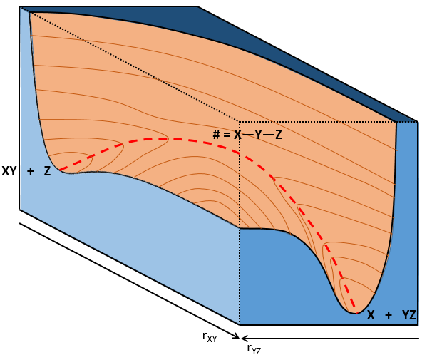
The path requiring the minimum energy is plotted in red and is called the reaction path and is the most probable path. Between the XY + Z and the X + YZ states, there is a state of transition # in which the liaison between Y and Z is not completely made and between X and Y not totally broken. The liaisons are extended and require more energy. Indeed, this state, called a complex of transition, is higher in energy than the state XY + Z and X + YZ. It is a saddle point in the space of reaction: a maximum in a direction and a minimum in another direction.
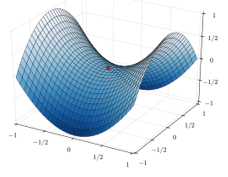
When the reaction reaches the transition state, the reaction can either go ahead or go back. The direction the reaction takes depends on the vibration and on the difference of energy between the states the reaction leads to. We can also represent the surface at two dimensions with isocurves of energy (see next figure).
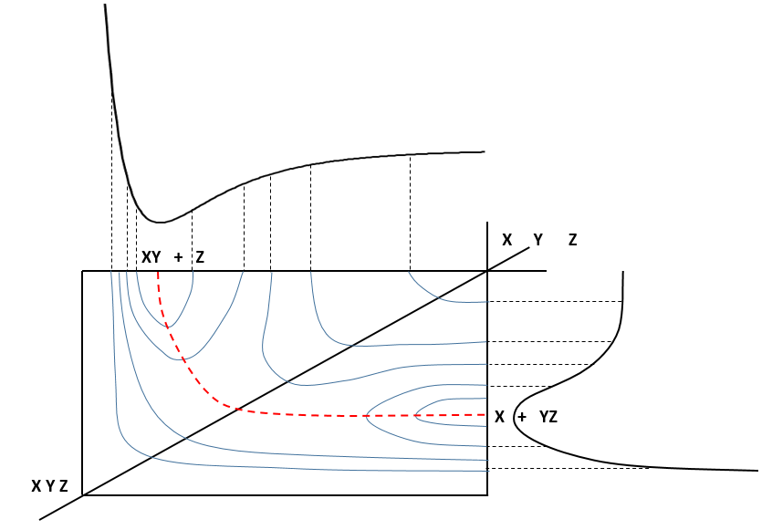
On the top side and on the right side of the graph, we see the potential curves of the liaisons YZ and XY respectively. The dotted line on the graph shows the path of lowest resistance. It is the most probable path of reaction. At the intersection between the axes, all three species are separated by the same, long distance and are not bound together. At the other side of the graph, there is no liaison between the atoms but they are very close to each other. If we plot the line connecting those two corners, the complex of transition is at the minimum of energy on this line.
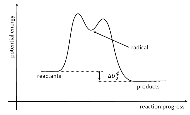
If we plot the potential energy along the reaction path, we will obtain something like this:
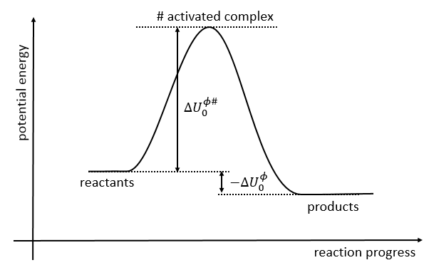
The ϕ symbol indicates that we are in normal conditions of temperature and pressure.
The model of the transition state
An equilibrium is considered to exist between the reactants and the complex of transition X#. From the complex of transition, products are formed with a frequency υt.
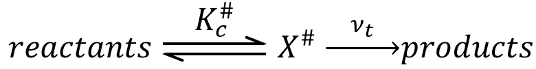
The speed of formation of the product is given by
![]()
Our problem is to determine the concentration of the complex of transition. We find it from the first step of the reaction. If this step is monomolecular (one reactant A), then
![]()
If the first step is bimolecular, then
![]()
If we replace υt Kc # by km, we find the experimental constant of reaction. To be perfectly correct,
![]()
where κ is the coefficient of transmission that is usually equal to 1.
Statistical formulation of km
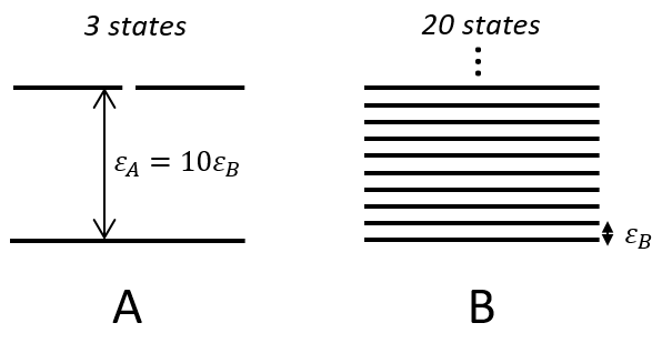
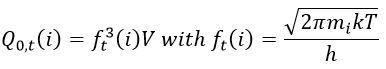
There is a given number Q of states that are accessible to each molecule.
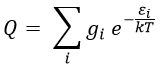
where gi is the degeneration of the state i and εi is the difference of energy between the state i and the ground state. The number of accessible states depends on the temperature.
where ΔU0 is the difference of standard intern energy with regards to the zero point. We can also consider the molar standard intern energy but in this case we have to divide the functions of partition Q0(i) by A0V, A0 being the number of Avogadro.We can link the equilibrium constant of a reaction with the functions of partition of the molecules that take part in the reaction. Let’s consider a reaction
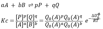
As km=υt Kc#, we can write
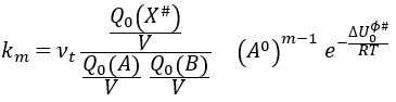
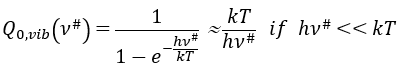
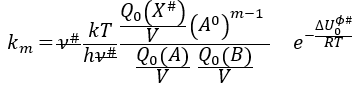
with m the order of the reaction. The function of partition of a molecule is related to its vibration, rotation and translation modes. For the complex of transition, the function of partition of the vibration mode can be isolated and is related to the frequency of vibration of the liaisons that are broken and made.
The function of partition is thus approximatively
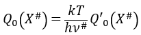
If the factor of frequency υt = υ#, then we obtain the statistical formulation of the constant of speed
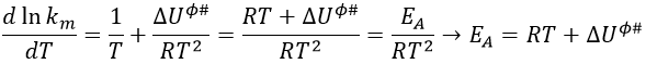
Q0(A) and Q0(B) can be determined by spectroscopy but Q0# has a life time too short to be correctly analysed (the time of a vibration, τ~100 femtoseconds). The functions of partitions depend on the temperature and we can globally write that
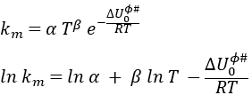
Taking the derivative of this expression with regards to the temperature, we obtain
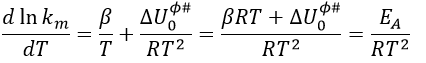
If we compare this expression to the law of Arrhenius, we have that
![]()
β is usually small so EA»ΔU0ϕ#.
Estimation of the pre-exponential factor of the equation of Arrhenius
We will consider the reactants as hard spheres.
![]()
In this condition, there is no vibration nor rotation to consider for them. They have thus only 3 freedom degrees. The function of partition of translation is
The transition complex is composed of two hard spheres and can thus rotate in two planes. We will assume that we can write the rotation and translation as two independent functions.
![]()
The mass we consider for the transition complex is simply equal to the sum of the mass of the two reactants: mAB#=mA+mB. The function for the rotation is
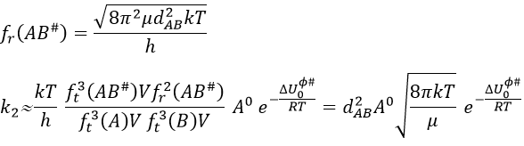
This expression for k2 is the same than the one obtain by the model of collisions but we obtained it with a totally different approach. As in the model of collisions, the molecules were considered as hard spheres and the model is not correct for more complex structures.
Thermodynamic formulation of km
In a gaseous phase, we have that
![]()
To obtain km in solutions, we have to divide Kc# by a power of the concentration cϕ=1mol/l
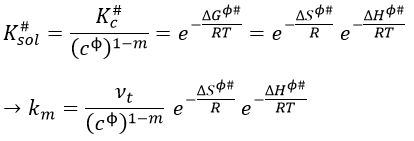
We want to connect this expression to the relation of Arrhenius. To do so, we need to make the approximation than υt=kT/h. As a result,
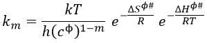
We will assume that ΔHϕ# and ΔSϕ# don’t depend upon T so that we can derivate the expression with regards to the temperature.
The enthalpy ΔHϕ# is related to the intern energy of activation ΔUϕ#. For ideal gases the relation is
![]()
Once the derivation d/dT is done, we obtain
Previously in the theory of the transition state, we found EA= ΔU0ϕ#+βRT. Here β=1.
The variation of entropy is thus included in the pre-exponential factor. There is a variation of entropy during the formation of the complex of transition. For unimolecular reactions A → B in gaseous phase, the variation of entropy is approximatively equal to zero as there is no variation in the number of particles.
If the experimental pre-exponential factor is larger than 10-13s-1, it means that there is a variation of entropy during the process and that the reaction is a reaction of dissociation (A → B + C).
The fact that the variation of entropy is present in A is a big advantage with comparison to the model of collision where a steric factor was considered to obtain a result similar to the experimentations.
Femtochemistry
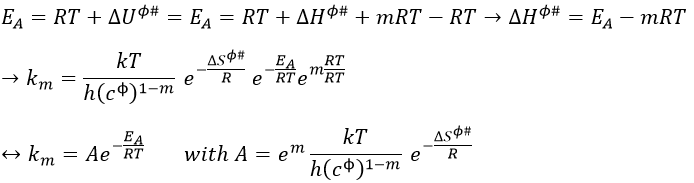
The femtochemistry allows to detect events with a timescale of the femtosecond. A. Zewail (Nobel prize in 1999 for his work on femtochemistry) studied in 1996 the transition states of chemical reaction with femtosecond spectroscopy. Using a rapid ultrafast laser technique (ultrashort laser flashes), the technique allows the description of reactions on very short time scales – short enough to analyse transition states in selected chemical reactions. For instance we can obtain 2 ethylene molecules from one cyclobutane and we want to determine the process. One possibility is the simultaneous cleavage of two liaison during one single vibration.
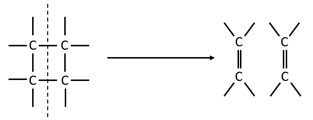
A second possibility involves the formation of a complex of transition wearing two radicals from the cleavage of one of the liaisons, and then the cleavage of the second liaison to obtain two ethylenes.
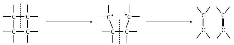
The second step of the reaction would be easier than the first step because the radicals help to the cleavage of the other liaison. The correct process is the one involving radicals. The life-time of the complex of transition is about 700fs and can be detected with femtosecond spectroscopy.
Application: photoreduction of the RuTAP by the GMP
We study here the transfer of one electron between the two species. The Ru(TAP)32+ (TAP= 1, 4, 5, 8-tetraazaphenanthrene) is a complex of coordination that can interact with DNA. We will next call it RuTAP.
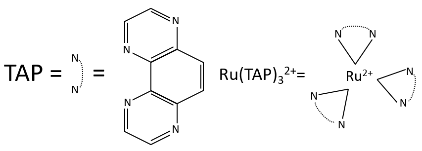
RuTAP absorbs in the visible (max at 420nm, orange-red).
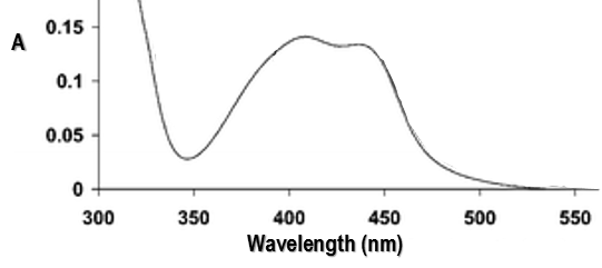
Instead of the analysis of the interaction of RuTAP with DNA, we replace the DNA by GMP (guanosine-5’-monophosphate) in this experiment. If we put RuTAP and GMP together in the dark, nothing happens. To observe a phenomenon, RuTAP has to be in an excited state. We illuminate the system at 420nm to excite RuTAP into RuTAP*.
![]()
The excited species will go back to its ground state through two possible reactions:
- the emission of a photon (not the same wavelength than the absorbed photon)
- the transfer of energy to the GMP. It leads to transitory products.
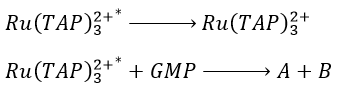
We want to determine the nature of A and B. We place the system in conditions such as the deexcitation through the emission of a photon does not occur. The illumination is only maintained during approximatively 10nanoseconds. However, the transfer of electron is completed over this period of time. After the pulse of light, we can study the evolution of the system through the emission of the solution. We don’t look at the wavelength in the range of the RuTAP (420nm) but in a range of frequencies where it does not emit: at 550nm, we find an intense signal that decreases quickly over time.
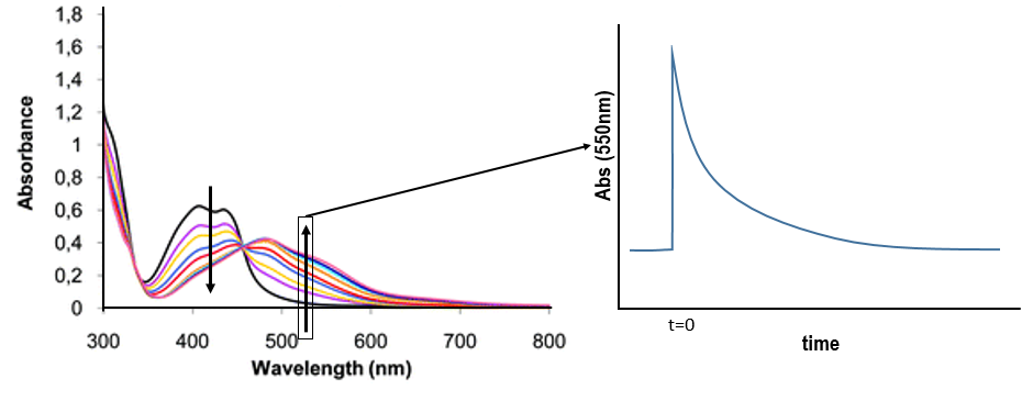
Before the pulse, nothing emits at 550nm. The formation of the emitting species is very fast but its decomposition is fast too. After the pulse, the transitory products of the reaction disappear over time and the signal comes back to zero. One hypothesis is that A is the reduced complex and that B is the oxidised GMP, respectively noted A=Ru1+ and B=GMP.+. This hypothesis is verified by a parallel experiment in which we measure the spectrum of Ru1+ alone.
We still meet one problem: the experiment was performed in a solution saturated in N2. When we repeat the experiment in presence of oxygen, the signal differs: the decrease of intensity is faster but the absorbance does not reach zero.
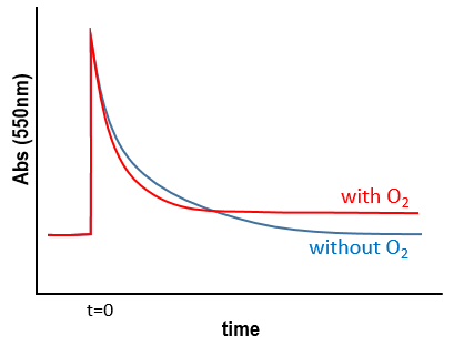
The oxygen generates an interference. To understand what happens, we analyse the signal in presence and in absence of oxygen. If we consider a monomolecular reaction, the decay should have the form of an exponential.
![]()
The characteristic time of this process is τ=1/k1. This type of decay is found in presence of oxygen (plus the fact that there is still a signal after the reaction).
If we consider a bimolecular reaction, with the same concentration for both reactants, then the decay is different.
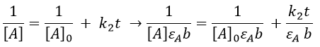
If we pose that k2’=k2/εAb, then

This decay is observed in absence of oxygen as expected for a reaction with two reactants
![]()
Note that we talk about equimolar reactants but the quantity of RuTAP and GMP that we put in solution at the beginning of the experiment does not matter. GMP.+ and Ru1+ are equimolar. The absorbance goes thus back to zero.
In presence of oxygen, there is a competition between the oxygen and the GMP.
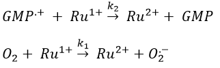
If the solution is saturated in oxygen (or if the system is open), then [O2]»constant and we find a pseudo order 1. This reaction occurs more than the reaction with GMP.+ because k1[O2]>>k2[GMP.+]. The signal does not go back to zero because some GMP.+ remains in solution (with a long life-time in comparison to the reaction). It is possible to determine the constants of speed k1 and k2 if we place ourselves in good conditions.
Chapter 8 : chemical kinetics – orders of reaction
Kinetics is a field of the chemistry that studies the evolution of a chemical process over time. It gives practical information on the reaction and can help to determine its mechanisms. There is already two chapters discussing the basics of kinetics (1, 2) and we will now explore a bit deeper this field of chemistry. A chemical reaction can be written
![]()
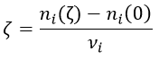
Where A, B, C and D are chemical species and υI is the stoichiometric coefficient related to the species I. The reaction can be an elementary reaction or a complex reaction composed of several steps. The advancement of the reaction ζ can be followed by the variation of the amount of one species i.
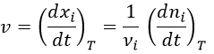
We can choose any species involved in the reaction as the studied species. The speed of reaction is given by the derivative of the advancement of the reaction at a given temperature. As we want only one characteristic speed of reaction, we divide the derivative by the stoichiometric coefficient of the studied species. Also note that products are formed while reactants are consumed. To have a positive speed, a minus sign is added if the studied species is a reactant.
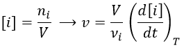
Instead of the amount of particles ni, their concentration is followed. Note that the volume is thus part of the equation but it is generally constant.
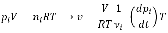
Instead of the concentration, we can use the partial pressure for gases.
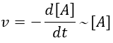
Experimentally, we will thus measure the concentration or the pressure of one species over the time. The concentration of a product increases over time while the concentration of a reactant decreases. The speed is defined positive and a minus sign must thus be placed before the derivative of the concentration of a reaction.
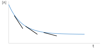
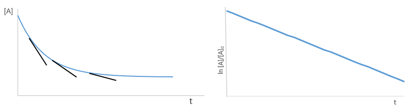
Yet, the speed of the reaction depends on the time: while approaching the end of the reaction, there is less reactant in the solution and the probability that the molecules of reactant are in contact so that they can react decreases. We want thus a measure that is independent of the time and characteristic of the reaction. On a graph of the concentration versus the time, the speed is proportional to plus or minus the slope of the curve. Obviously the slope changes over the time.
Reactions can be subdivided as a function of the order of reaction.
Reaction of first order
![]()
It is for instance a reaction of decomposition or a catalysed reaction. k1 is the constant of equilibrium, with 1 as index to suggest the order of reaction. A is one reactant and B is one product of the reaction. The instantaneous speed is directly proportional to the instantaneous concentration.
The coefficient of proportionality is the constant of speed k1.
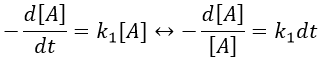
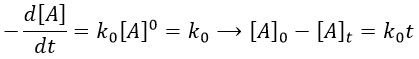
The units of k1 are s-1: when we look at the equation, [A] and d[A] have the same units –mol- and dt is in s. Each side of the equation has to have the same units so k1 is in s-1. The resolution of the equation is
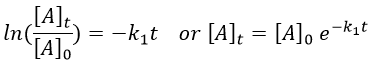
with [A]0 and [A]t respectively the initial concentration of the reactant and its concentration at time t. The concentration decreases exponentially over the time but we can plot the logarithm of the concentration ln[A] as a function of the time to find a straight line the slope of which is –k1.
If instead of measuring the evolution of the concentration of the reactant we measure the evolution of the concentration of the product B, we know that both concentrations are related. The amount of B that is formed is equal to the consumed amount of A, i.e. the initial amount of A minus the amount of A that is still in solution. If there was no product is solution at the beginning of the reaction, then our final concentration of product will be the initial concentration of the reactant.
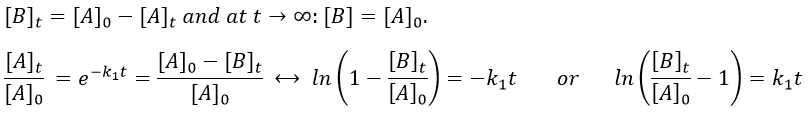
We can thus also find a straight line the slope of which is k1.
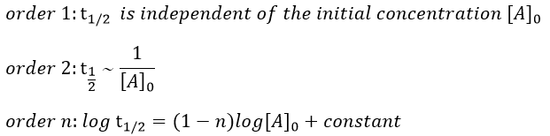
A time of half-life, i.e. the time required for the consumption of half of the reactant A, can be determined. It is not equal to the half of the time required to consume all the reactant.
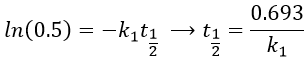
This time is independent of the initial concentration. After t1/2, the concentration of reactant is divided by 2. After 2 t1/2, the concentration is divided by 4. After 3 t1/2, by 8, etc. The measurement of those times we can confirm the value of k1 that was found by the slope of ln [A].
The concentration can be followed by a measure of the absorbance of the solution, of its pH, conductivity or optical activity.
Reaction of order 2
If we consider only one reactant and we don’t find the previous relations, the reaction can be of a higher order than the order 1. Two identical molecule can merge to form one new product, by condensation for example (amino acids).
![]()
In this case, the speed of reaction depends on the square of the concentration of the reactant.
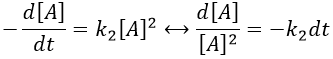
Note that this constant of reaction k2 has not the same units that the constant of reaction k1 of reactions of order 1. In d[A]/dt=k2[A]2, we have the square of a concentration at one side of the equation and a concentration at the other side (with a variation of time). The units of k2 are mol-1s-1. If we consider a gas, we will follow the pressure pA of the reactant.

As a result,

In a general way, we have kmp=kmc(RT)m-1 with m the order of the reaction.
The solution of the equation
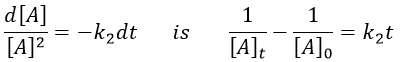
If we plot the logarithm of the concentration, we won’t find a straight line this time. To obtain one, we have to plot 1/[A]. The slope of the line is the constant of speed of the reaction.
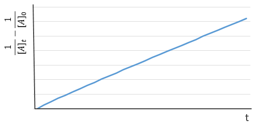
The half-life time is obtained from

This time, t1/2 depends on the initial concentration of the reactant. The half of the concentration is consumed over t1/2. The time to consume half of the remaining concentration [A]0’ (i.e. to consume the next [A]0/4) is not the same time but twice as long because the initial concentration is now [A]0’ and is the half of the initial concentration [A]0.
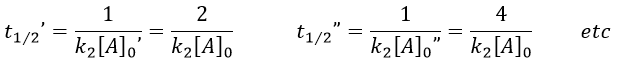
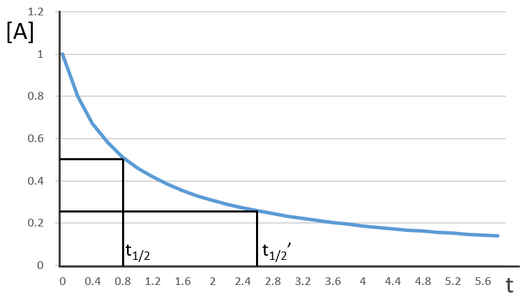
The half-life time becomes longer and longer with the advancement of the reaction.
Reactions of order 2 can also involve two different reactants.
![]()
A and B are consumed at the same rate but the concentrations can be different if there was an excess of one of the reactants.
At a given time, a concentration x of A and of B has been consumed by the process. We can thus replace the concentration at that time by the difference between the initial concentration and x.
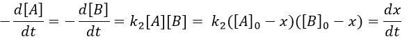
From two parameters we have now only one parameter, x and the equation can be solved.
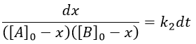
We can integrate the equation over the time of the reaction (from t=0 to t and from x=0 to x).
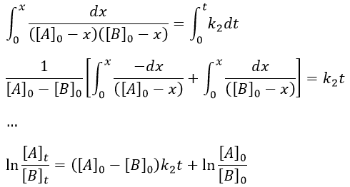
If [A]0=[B]0, then the ratio of concentrations [A]/[B] always remains constant but we won’t be able to determine k. The trick is to put one reactant in large excess and to follow the concentration of the second reactant. If one reactant is put in excess, then the expression for the concentration is more complicated. But if we put an excess large enough to consider the concentration of the other reactant as negligible, then
![]()
Then we obtain a pseudo-order 1 reaction.
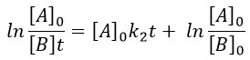
The second logarithm can be moved in the first:
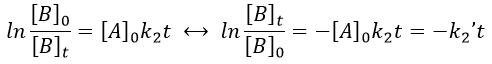
with k2’=[A]0k2 a kinetic constant of (pseudo)order 1. As we can find k2’, we know k2=k2’/[A]0.
The bimolecular nucleophile substitution (SN2) is a reaction the mechanism of which was found by regular kinetics studies.
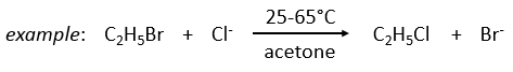
On the other hand the SN1 reaction showed extravagant results during the kinetics studies: the speed of the reaction was independent of the initial concentration of one reactant.
Reactions of order 0
In this kind of reaction, the speed of reaction does not depend on the concentration of one or more reactants.
It is typically the case when the reaction is made through several steps. We also find order 0 if there is a limiting factor such as the surface of a catalyst. The speed of reaction is then constant over the time. If we take the case of one SN1, the reaction involves 2 reactants but does not show the expected order 2 for the reaction.
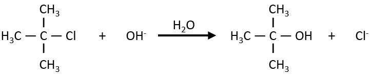
The reaction shows a kinetics of order 1 with regards to the chlorobutane and order 0 with regards to the hydroxide. The reason is that the reaction is made in two steps and the determining step is the first step in which OH– takes no part. The first step involves the formation of a carbocation from the chlorobutane, i.e. a reaction of order 1, and then a reaction of the second order that is much faster than the first reaction.
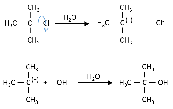
As the second reaction is much faster than the first, it is not this reaction that limits the global speed of reaction and we detect experimentally only the first reaction that does not include OH–. We can verify the order 0 by putting a large excess of the alkane in the solution and measure the evolution of OH–. It will decreases proportionally to the time and confirm the order 0.
An example of the utility of the kinetics is the synthesis of glycerol starting from epichlorohydrin made by Ernest Solvay.
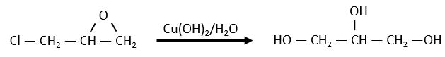
The glycerol and the epichlorohydrin are both transparent but once the reactant were put in the reacting tank and heated the system, the solution turned yellow-brown. They though that they overheated the system but it was still the same with a lower heating. A PhD in kinetics was consulted on the subject. He found out that the reaction is of order 0 with regards to the epichlorohydrin, meaning that the reaction involves several steps. If they heated up the reaction, they found an order 1 reaction. In fact, there is a determining step before the reaction: the dissolution of the epichlorohydrin into water.
As we have seen, a reaction can have a different order depending on the observed reactant. The global order n of the reaction is the sum of the orders with regards to each reactant.
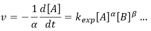
Where α, β, … are the order with regards to A, B, … and n=α+β+… is the order of reaction. There are several methods to determine experimentally the orders of a reaction with regards to the reactants
Method of integration
This method uses the relation between the evolution of the concentration of one given species over the time to determine the order of reaction with regards to this species: we verify if we can obtain a straight line on the graph of ln[A] vs time (order 1), of 1/[A] vs time (order 2) or of [A] vs time (order 0).
Method of half-life time fraction
We use here the properties of the half-life time if the reaction speed only depends on one of the reactants (the others are put in excess). We vary the initial concentration of the studied reactant.
Method of isolement
All the reactants except one are in excess. We measure the order of the reaction with regards to this reactant.
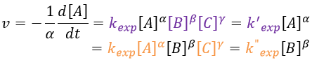
We proceed the same way with a different reactant (no excess of concentration) to determine the pseudo-orders of reaction with regards to each analysed reactant and we combine the result to find the order of reaction.
Method of the initial speeds
As usual we measure the evolution of the concentration as a function of the time. The tangent of the curve at t=0 gives the initial speed v0 (-v0 to be accurate). One reactant is not put in excess and is measured.
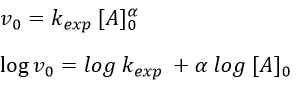
The experiment is repeated several times (it is quick because we only look at the beginning of the reaction) for several initial concentrations. This way we can determine kexp and α. This method is not very accurate because we measure a tangent at t=0.
When we study the kinetics of a reaction, we must always at least use the method of integration and of initial speeds and obtain concordant results. If it is not the case, the supposed mechanism is not correct.
Chapter 7 : MPC – Molecular degrees of freedom: vibration and rotation
In the Born-Oppenheimer approximation, we froze the position of the nuclei to find the electronic energy. The position of the nuclei was considered as a parameter that can be modified and we were able to construct the Lenard-Jones potential for the liaisons or the surface (or hypersurface) of potential energy for molecules with more than one liaison. We will now discuss in further details about the vibration and rotation modes of molecules ant thus incorporate the movements of nuclei in the model.
The first step is to choose the set of coordinates in which we will work. A molecule with M nuclei has 3M coordinates: (xi,yi,zi) for each of the M atoms.
The laboratory axes system (LAS) is the first set of coordinates that we use. In this system we determine the position of the centre of mass of the molecule. Those 3 coordinates allow us to determine the translation of the molecule but not the rotation or the vibration modes: the centre of mass doesn’t move because of those modes.
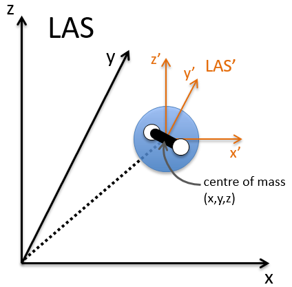
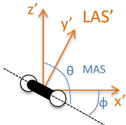
To determine those modes, we need two other sets of coordinates: the LAS’ that is fixed to the centre of mass of the molecule and consequently is independent of the translation and the MAS: molecular axes system that is fixed to the molecule and turns with it. 2 angles 0≤θ≤π and 0≤Φ≤2π are used to locate the linear molecules and a third one 0≤χ≤2π is needed for the nonlinear molecules. Those 3 angles are called the angles of Euler and are
From the 3M coordinates, we used 5 (linear molecules) or 6 (non-linear molecules). The rest correspond to the modes of vibration of the molecule. In a diatomic molecule, there will be only one mode of vibration: M=2 and 5 coordinates are used to locate it.
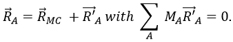
To resume, the coordinates of one molecule are given by the vector
![]()
with 3M dimensions. The translation of the centre of mass is determined in the LAS
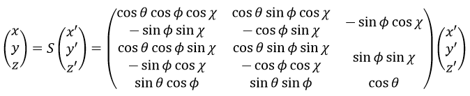
The condition here reflects the facts that the centre of mass does not move in the LAS’ referent. The MAS rotates with the molecule. To move into this referent, we apply the matrix S to the vector RA’.
![]()
The matrix S defines the orientation of the axes (x’,y’,z’) of the LAS’ from the coordinates (x,y,z) of the LAS:
Small vibrations around the equilibrium RAeq are given by the vector dA
![]()
with the conditions of Eckart that
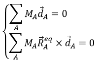
The first condition reflects that the centre of mass does not move because of the vibration and the second condition that there is no rotation in the MAS.
The kinetic energy of the molecule is in this notation
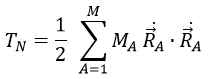
with MA the mass of the nucleus A and ṘA=dRA/dt. Replacing ṘA by its expression
![]()
We obtain (the red terms equal zero)
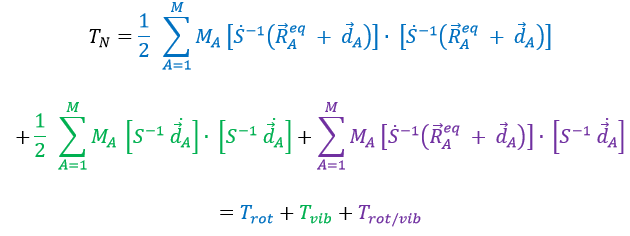
If Eckart is respected, then the interaction term Trot/vib can be neglected. We can thus approximate that the energies of rotation and of vibration are separable. The order of magnitude is indeed different: the vibration is found into the infrared while the rotation is observed in the microwave range.
![]()
Vibration
For a diatomic molecule, the oscillation is characterised by a force of recall
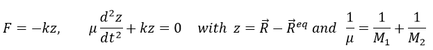
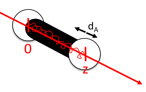
We find that
The energy of vibration can thus be approximated to a constant. The kinetic energy Tvib is always positive and is thus equal to
![]()
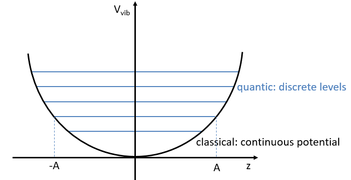
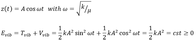
From the quantum mechanics, we know that
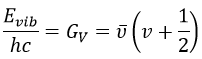
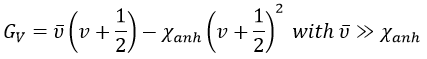
The separation in energy between the levels characterised by a number of nodes v=0, 1, 2, … There is thus regular a ΔGV=ῡ.
There is however a deviation to the harmonicity that we found. If we develop the potential as a series of Taylor, we obtain
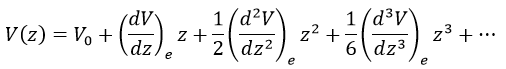
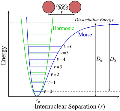
The two first terms are simply equal to zero (V0=0 and the potential is at a minimum at the equilibrium). The third term is the harmonic result that we just obtained but further terms express the deviation to the harmonicity. The potential of Morse gives an empiric formula that fits correctly the real potential.
![]()
The anharmonicity modifies slightly the energy of the states
In the case of polyatomic molecules, we can consider that all the nuclei oscillate in phase, giving a base of 3M-6(5) independent movements. The result doesn’t noticeably differ from the diatomic molecule in this case.
Rotation
The rotation can be considered as a rigid rotation: the difference of frequency and of energy between the rotation and the vibrations is huge enough to make this approximation. The angular speed ω is thus identical for all the nuclei of the molecule.
![]()
The kinetic energy due to the rotation for a diatomic molecule is thus
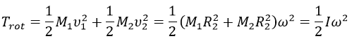
with I the moment of inertia that is common to the two atoms.
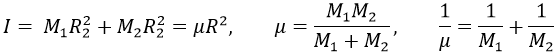
μ is the reduced mass of the molecule. The angular moment J is given by
![]()
Its absolute value is
![]()
For a diatomic molecule, we get
![]()
The angular moment and the kinetic energy are thus directly bound:
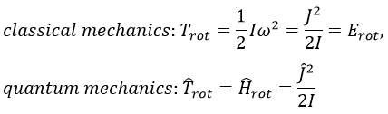
We can go from the classical mechanics to the quantum mechanics by the application of the Hamiltonian on a wave function.
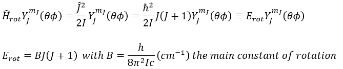
The multiplicity is gJ=2J+1. A small correction has to be added due to the centrifugal distortion, correction which is normally very small and negligible except when the rotation is very fast:
![]()
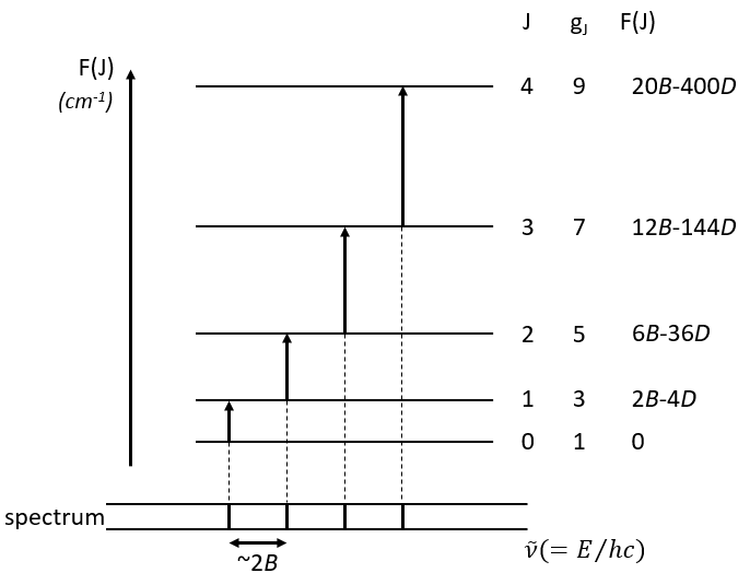
The spectrum of the rotation is thus composed of bands regularly spaced.
Chapter 6 : MPC – The LCAO theory
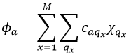
This theory says that each molecular orbital Φa is described by a linear combination of atomic orbitals {χ} centred on the M nuclei of the molecule.
The molecular orbitals have the symmetry of one of the irreducible representations of the group G. This symmetry is taken into account in the LCAO coefficients. Some are null (some symmetries are not used) and some are equals in absolute value: only functions of same symmetry interact together to form molecular orbitals.
Given a MO Φa ∈ D(i) of G and the AO {χ}, we can adapt the atomic orbitals to the symmetry of D(i): {χ}à{χ(i)}. Then
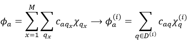
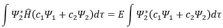
The advantage of doing this is that the number n(i) of functions χ(i) in the last expression is smaller than (or equal to) the number n of functions χ in the atomic orbitals. Let’s apply the LCAO theory to an example in which the orthonormal base is composed of two function {Ψ1, Ψ2}, i.e. a case where two states are in interaction with each other.
![]()
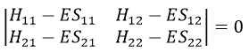
The secular determinant is
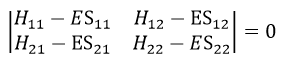
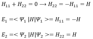
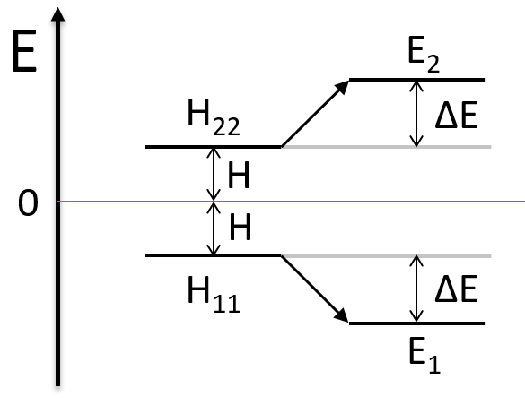
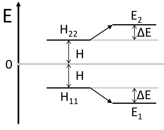
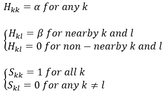
As the base is orthonormal, S is a delta of Dirac: S12=S21=0, S11=S22=1 and H12=H21. Posing that the two states H11 and H22 are equidistant from the zero energy, they are separated in energy by 2H:
We can represent the problem as follow:
The secular determinant is thus reduced to
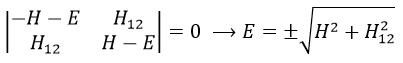
and
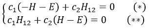
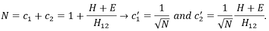
If we set c1=1, then c2=(H+E)/H12. The coefficients must still be normed.
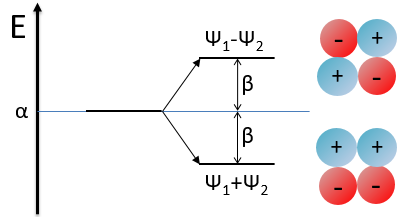
Two cases can be considered:
- H=0 with H12<0.
Two degenerated states interact with each other. The result of this interaction is that the states are repelling from each other. One is stabilised and the other one is destabilised by ΔE=H12. We will obtain a bonding state and an antibonding state. H12 is thus a measure of the interaction between the states. The bigger it is, the bigger is the separation between the resulting states. H was the distance between the states that interact together.
![]()
Posing that c1=1, then c2=-1. The coefficients must still be normed: c1=1/√2 and c2=-1/√2. As a result, the wave function of the state of energy E=-H12 is
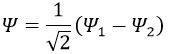
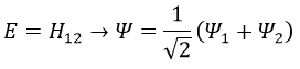
We can do the same for the second state (E=H12) and obtain
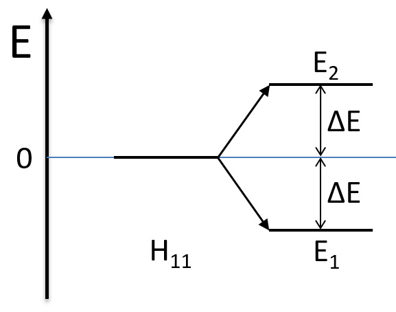
- H≠0 and H>>H12
The states that are interacting together have not the same energy. For instance, let’s consider H=2 and H12=-1/2.
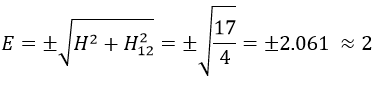
The interaction between the two states separated the states but just by a bit. The states did not mix a lot together.
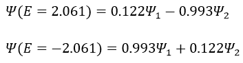
The mixing between two states is inversely proportional to the difference of energy between the states.
If H12=0, there is no interaction between the states. It is the case only when the states don’t share any symmetry, i.e. H12 can be different from zero only if Ψ1 and Ψ2 have common proper values with all the operators that commute with Ĥ. As a result, a triplet does not interact with a singlet even if the energies of those states are similar.
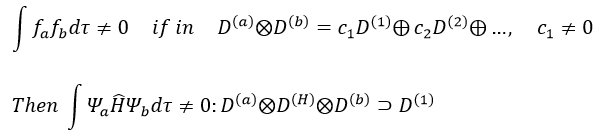
Rule of non-cancellation of an integral:
An integral is not equal to zero if the integrand is invariant with regards to all the operation of the group G, i.e. if the reduction of the direct product contains the totally symmetric irreducible representation D(1). In other words, the integral is different from zero if the integrand is totally symmetric.
Cases of H2+ and H2
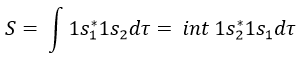
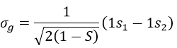
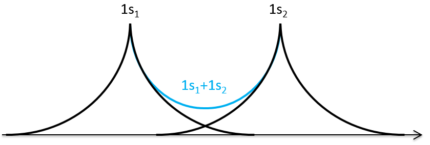
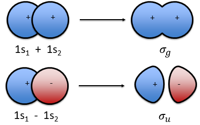
The orbitals 1s of the two atoms are interacting together to form molecular orbitals σg and σu. σg is a binding orbital resulting from a constructive interference:
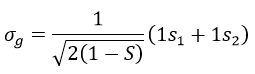
Here we considered that the base is not orthonormal. It is why the norm is 1/√(2(1-S)) and not 1/√2. S is the deviation to the orthonormal base
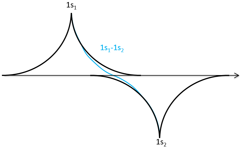
In an orthonormal base, S=0. The antibonding state σu is resulting from a destructive interference
The interactions can be seen this way:
When the electron is in a molecular orbital such as the attraction it produces on both nuclei brings the nuclei closer to each other, the effect is binding.
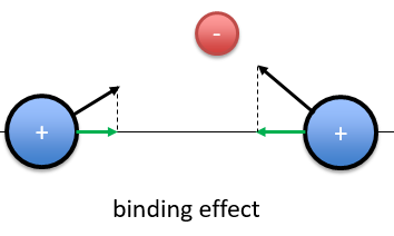
In the figure above, the electron is between the two nuclei. The attraction is produces on the nuclei is represented by the black arrows. The green arrows are the projection of the attraction on the axis passing by the two nuclei. The nuclei move thus in the direction of the other nucleus and remain thus together because of the presence of the electron.
If the position of the electron leads to a separation of the nuclei, then the effect is antibonding. The interaction of the electron-nucleus is positive but the intensities and directions are such as the nucleus-nucleus distance increases.
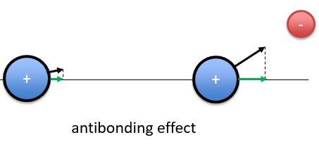
In the picture above, both nuclei are attracted by the electron but they move in the same direction with different speeds. The nucleus of the right moves faster than the nucleus of the left and the nuclei move thus away from each other.
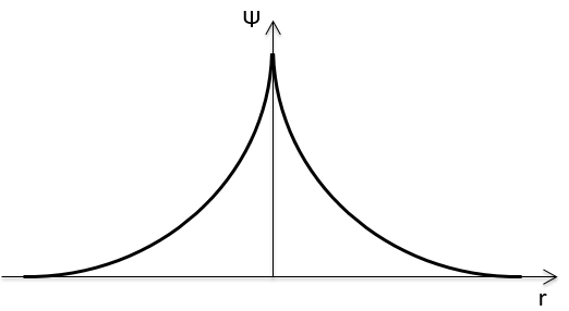
The function 1s can be expressed as an exponentially decreasing function centred on the nucleus.
We can superimpose the functions 1s of two hydrogen atoms. In the case of σg, the functions add together:
We can do the same for σu.
If we put those function to the square, we obtain the probability of presence of electrons.
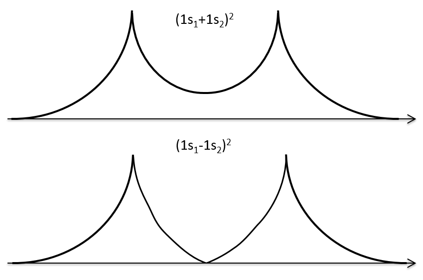
In the second case, there is a place between the nuclei where no electron can be found. No liaison can thus be done between the nuclei.
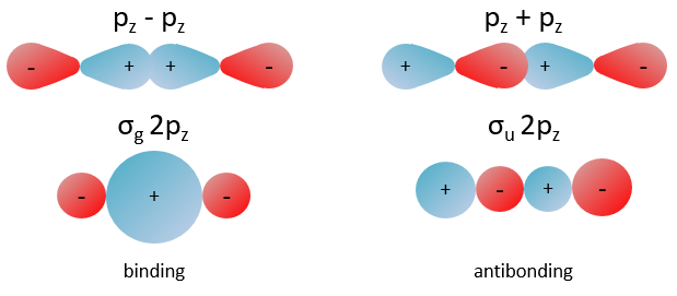
Interaction between 2p orbitals
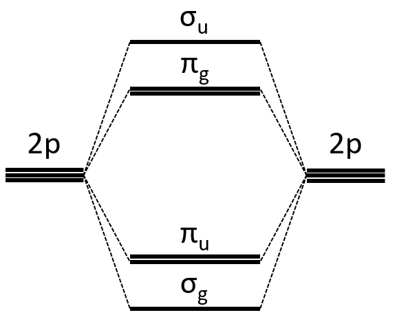
All the 2p orbitals don’t interact the same way. The 2pz orbitals interact together to give the σ orbitals. This time, it is not the sum of the atomic orbitals that give the molecular orbital of lower energy and the binding orbital σg.
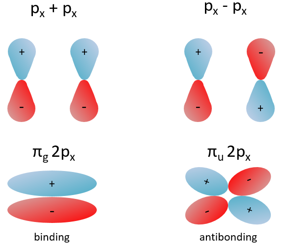
The other 2p orbitals (2px, 2py) lead to the π orbitals.
Note that the energy of the orbitals depends on the atoms. They all decrease in energy with Z but not with the same speed (see the figure below).
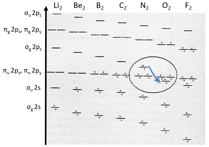
The energy of the πu orbitals is almost constant while σg 2px decreases quickly with Z. σg 2px falls under πu at O2.
The energy of the liaison between the two atoms increases up to N2 and decreases after because electrons are placed in antibonding orbitals.
The Walsh diagram
This diagram relates the energies of molecular orbitals of a molecule as a function of the angle that separates the liaisons. It helps to visualise the stability of the liaisons with regards to the symmetry of the molecular orbitals. The following figure shows the Walsh diagram for AH2.
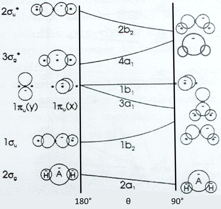
On the left one sees the linear molecules. As we go towards the right, the angle between the two liaisons goes towards the right angle, i.e. towards a bent conformation. As the bond angle is distorted, the energy for each of the orbitals can be followed along the lines, allowing a quick approximation of molecular energy as a function of conformation. As we move towards the top, the energy of the liaisons increases. Note that the 1πu orbitals are degenerated for an angle of 180° but separate if we change the conformation of the molecule.
For one molecule, we count the number of electrons of valence. For instance BeH2 has 6 electrons of valence (4 for Be and 1 for each H). We place 2 electrons by line, starting from the bottom (note that the 1a1 line, binding the σg orbitals, is not plotted. The last electrons are on the 1b2 line. One can see that the most stable angle for this molecule is 180°. For BH2 and CH2, the molecules are bent. If one electron is excited, then the conformation of the molecule can change.
Method of Hückel
This method limits the LCAO method to the π electrons. The reason is that a lot of physicochemical properties of the molecules can be explained by the π-π* orbitals. In the method of Hartree-Fock, the secular determinant was
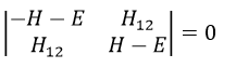
We have to solve the determinant for all the orbitals of the molecule, what can quickly become complicated. If we apply the method of Hückel on C2H4 for instance, there is only one π liaison in the molecule and thus only one secular determinant to solve. Considering two degenerated levels of energy α, the secular determinant is
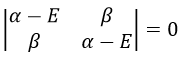
α=H11=H22 is the energy of the perpendicular to the plane atomic orbitals of the carbons and beta is the energy of resonance/interaction.
The solution found with this method (we won’t do it here) is close to the one obtained with the Hartree-Fock method that consider all of the electrons.
This method can be extended to other systems with π electrons if we pose that
If we consider the butadiene, we consider it as the interaction of two π systems
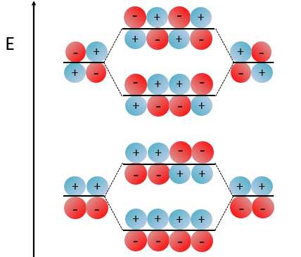
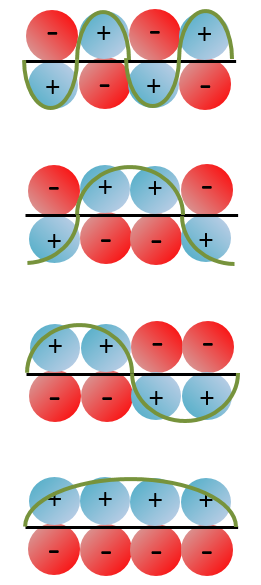
With the increase of π electrons, there are more binding states and one can see that, looking from the bottom to the top, the organisation of the orbitals follows a simple rule: the number of times that the signs are reversed increases by one at each orbital. One talk about the “wavenumber” of the orbitals. Indeed, on the lowest energy state, all the orbitals are aligned. There is no change of orientation of the orbital. On the second lowest state, the two orientations of the orbitals are present but they are grouped. There is only one change of orientation. The third level has 2 changes of orientations, there are 3 changes on the fourth lowest state, 4 on the fifth, etc… If we look at the orbitals as a wave, the wavenumber is indeed increasing with the energy of the state.
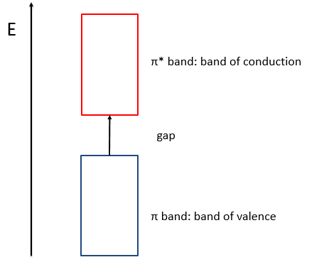
When the amount of π liaisons increases,
- the separation in energy between the states of same type (binding or antibonding) decreases and for a large amount of liaisons (in polymer for instance), we talk about a band of valence for the block of binding states and about a band of conduction for the block of antibonding states, separated by a gap.
- the amount of states increases in both bands,
- the separation in energy between the band of valence and of conduction decreases.
Chapter 5 : MPC – The methods of approximation and the quantic chemistry
We have seen quite a lot of new stuff up to now. We described monoelectronic and polyelectronic atoms and developed the description to molecules through the approximation of Born-Oppenheimer, the theory of groups and the CSOC. All of this teaches us how orbitals are and how they change during a reaction. Yet, we did not find the energies of the orbitals and can’t say which one is more stable than the others. The general equation is, as seen at the beginning of the course,
![]()
From the wave function we want to determine the energy of the orbitals but we can’t solve the equation exactly except for systems with one electron. For other species, we can only find an approached solution. To obtain it, we use the theory of perturbations or the method of variations.
Theory of perturbations
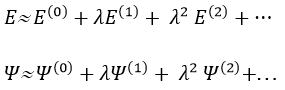
We can apply this theory to states that are independent of the time, i.e. stationary states. We can approximate the Hamiltonian and the energy of one state if this state is the result of a small perturbation λ of a state the solutions of which are known (Ĥ(0), E0).
![]()
The solutions are then expressed as a series of correction to the model at order zero.
The corrections are calculated from the solutions at the order 0. For instance, the correction of order 1 are
![]()
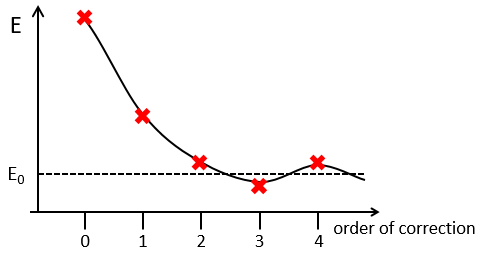
The corrections usually decrease in intensity with their order but they will always approach the approximation from the exact solution. Note that we can go beneath the exact solution.
Method of variations
To find the exact energy, we use a trial wavefunction. This function has a known form but will probably not give the exact energy but will give us a superior born for the exact energy. Next, we modify the parameters of the trial wavefunction to obtain a better approximation of the energy. Unlike the method of perturbation, we can’t go beneath the exact energy with the method of variations. Each time we modify the parameters, we obtain a solution of lower energy and we approach the exact value of the energy. For instance if we chose a wavefunction with two parameters α and β. We can try to improve the values of the parameters to obtain the best possible approximation.
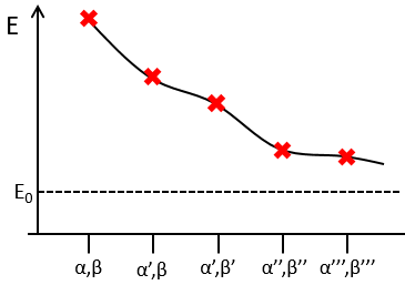
We reach an optimal estimation when the energy does not vary anymore when we change the parameters, i.e. when dE/dparameters=0.
Application to the helium
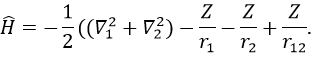
We will apply those two methods to estimate the energy of the helium. The exact solution is E=-2.903u.a. and the complete Hamiltonian is
One model the solution of which is known is the hydrogenous model:
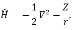
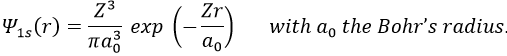
The solution of this model for 1 electron is
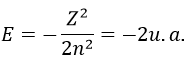
with Z the atomic mass and the quantic number n. As there are two electrons in the helium, we simply multiply the energy by 2 to obtain a first approximation from the hydrogenous model:
This approximation is far from the exact solution and overestimates the stability of the atom because we did not take the repulsion between electrons into account (the +1/r12 term).
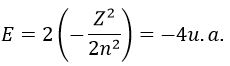
The theory of the perturbation will start from this model and introduce the repulsion term as a pertubation of the model:
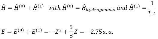
This estimation is way better than the hydrogenous model alone.
The method of variations is slightly different as we choose a wave function Ψ that depends on a few parameters that we may vary. As for the theory of perturbations, we select the hydrogenous wave function
As there are two electrons in the helium, we use a combination of two wave functions:
![]()
The parameter that we will vary is the effective charge Z=Zeff. One part of the charge of the nucleus is indeed hidden to one electron by the second electron.
From the chosen wave function, we find an equation for the energy that depends on Z
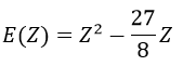
We optimise the parameter to obtain the best approximation that we can, such as dE/dZ=0. Solving this, we find
![]()
We apply this particular value of Z to the equation for the energy to find
![]()
This result is close to the exact solution.
Principle of linear variation: linear combination of atomic orbitals (LCAO)
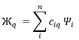
In this method, we assume that Ж can be expressed as a linear combination of a base of functions {Ψ1, Ψ2, …}
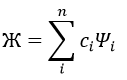
where ci is the variational parameter associated to the wave function Ψi. These coefficients are adjusted to approximate the exact energy. For more simplicity, let’s take an example in which Ж is a linear combination of two wave functions Ψ1 and Ψ2.
![]()
It is corresponding to the case of H2:
![]()
The Hamiltonian is
![]()
Next we multiply this equation by Ψ1* and integer it over tau:
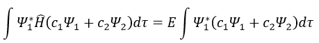
We can do the same with Ψ2*:
Now, we introduce Hij and Sij such as
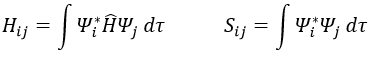
The previous integrals can be written
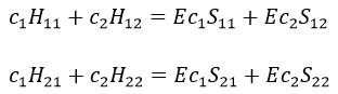
or
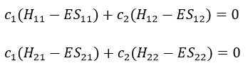
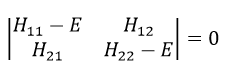
This system of two equations can be written as a 2×2 secular determinant
In a general way, it forms a n by n secular determinant if there are n wave functions (or particles)
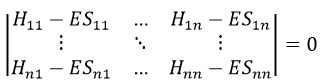
The n solutions of the secular determinant give the n most stable states of energy of the system. If we inject one of the energies E=Eq in the system, we obtain the optimised coefficients {ciq} related to the state q.
If the base is orthonormal, then
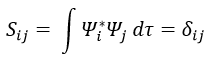
And then
If the base is complete, the linear combination corresponds to the exact solution due to the theorem of superposition (Quantum superposition is a fundamental principle of quantum mechanics. It states that, much like waves in classical physics, any two (or more) quantum states can be added together (“superposed”) and the result will be another valid quantum state; and conversely, that every quantum state can be represented as a sum of two or more other distinct states). The more the base is complete, the more one tends to the exact solution.
Method of Hartee-Fock
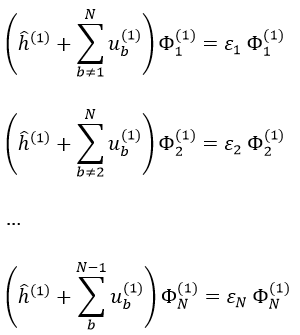
This method is an application of the variational method in which the trial wave function is a normalised determinant of Slater Ж = ∣ Φ 1 Φ 2 Φ 3… Φ N ∣. We try to minimise the energy of the orbitals (∂E/∂Φi=0) and to keep them orthonormal. We obtain a system of N coupled equations of Hartree-Fock that describe the movement of one electron in the averaged field ub created by the other electrons, such as
where εa is the HF energy of the molecular orbital Ψa. If we introduce the operator of Fock
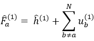
we can rewrite the system of N equations as
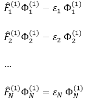
or on one line:
![]()
This equation only depends on the position and the movement of one electron, the effect of the other electrons being averaged. As the averaged field is determined by the orbitals that we are looking for, we have to solve the system of equations by iterations, starting from a set of orbitals of trial.
The convergence is guaranteed by the variational principle. In practice, we develop each orbital as a linear combination of Gaussian atomic orbitals centred on the nuclei. Then we iterate.
Chapter 4 : MPC – Orbital angular moment L
The electrons revolving on an orbital generate an angular moment.
ML is the quantic number associated to the projection of L on the internuclear axis.
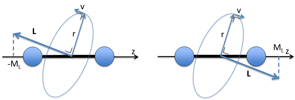
The projection is degenerated because it can either be in the positive values of the z axis or in the negative ones. The projection of L can thus give ML or –ML. We can define a new quantic number L=∣ML∣.
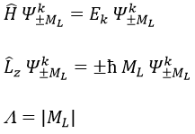
The fact that there are two projections explains the dimension 2 or the orbitals π, δ, … of linear molecules. The length of the projection of L grow if L gets larger but the degeneration is always 2. The only exception is Σ for which ML=0. In the atoms we had the possibility to choose the orientation but we cannot do that with molecules.
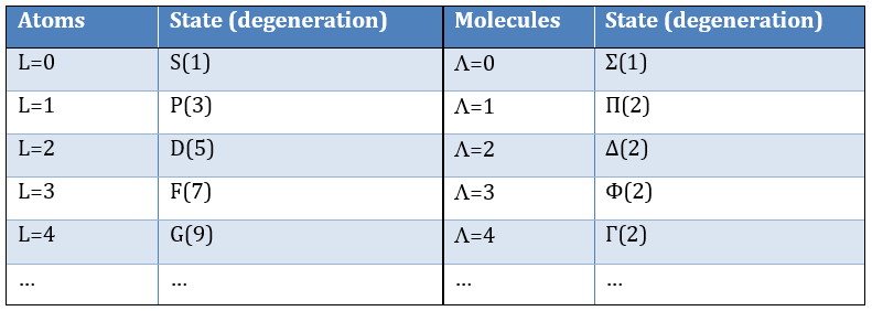
As a result, the operator σv doesn’t commute with Lz:
![]()
except for L=0 that gives the states Σ+ and Σ –. This distinction + or – is not present for the states Π, Δ, …
The fact that σv doesn’t commute with Lz induces the degeneration of the states.
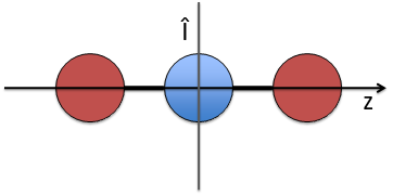
The inversion operator Î still commutes with Ĥ, Lz and σv in the case of centrosymmetric molecules.
![]()
As a resume, the operator σv is separated from the other operators of the CSCO of linear molecules because it does not commute with Lz anymore.
![]()
Application to H2
Let’s take a look at the possible electronic configurations of the molecule H2.
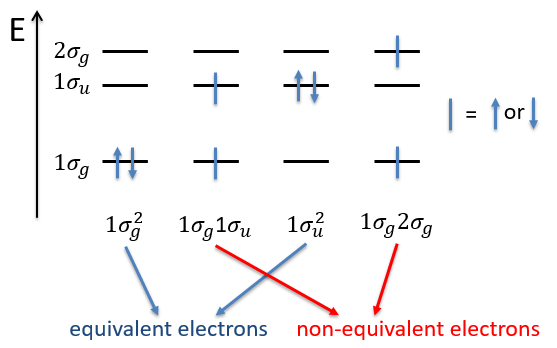
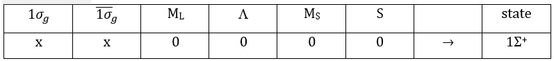
The unexcited state of H2 has two equivalent electrons on the ground orbital 1σg:
![]()
This state is binding: between the nuclei, the probability of presence of electrons is positive. In antibonding states, there are some points between the nuclei where the probability to find electrons is zero.
The first excited state is the configuration 1σg1σu. In this configuration the electrons are not equivalents and the degree of degeneration is 4 (2×2):
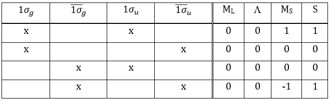
To determine the states, we take the emergent (ML=0,MS=1). It corresponds to the triplet 3Σ u + (the pairs (0,1), (0,0) and (0,-1)). The second emergent (0,0) corresponds to the singlet state 1Σ u +(the pair (0,0)).
To determine the energy of the states, we proceed as for the atoms with the determinants of Slater
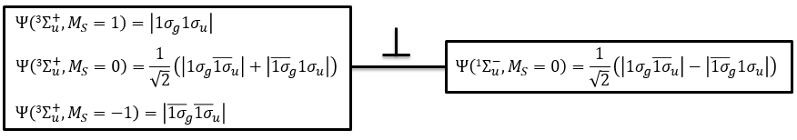
In the case of an emergent such as (0,1) we have a proper function and thus the energy can be determined. From this function we find the other functions with operators of rise/descent S+ and S– and with the principle of orthogonality we find the energy of the singlet state.
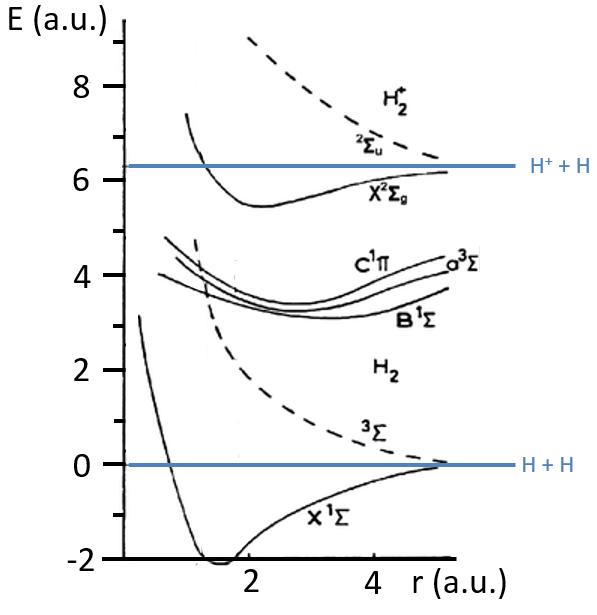
The dashed curves are correspond to unstable states because there is no minimum of energy: the atoms are get more stable as they get away one from each other.
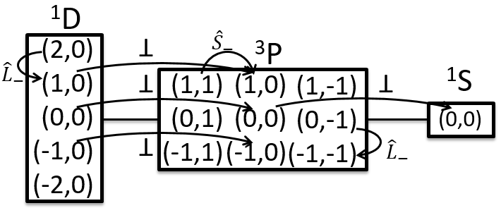
Application to O2
The same method can be applied to O2. Its fundamental configuration is
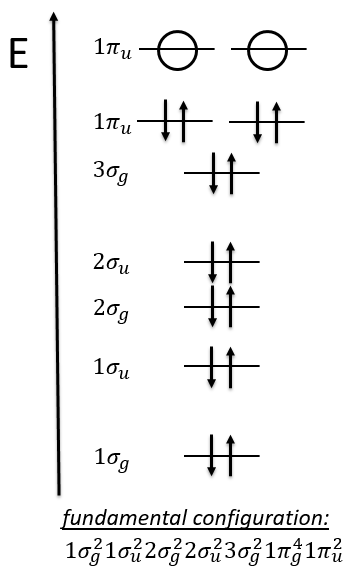
As usual, we only consider the highest occupied molecular orbitals (HOMO). Those are the 2 1πg orbitals with 2 electrons to place, represented above by the circles: they can be on the same orbital or separated. There is thus a degeneration of 6:
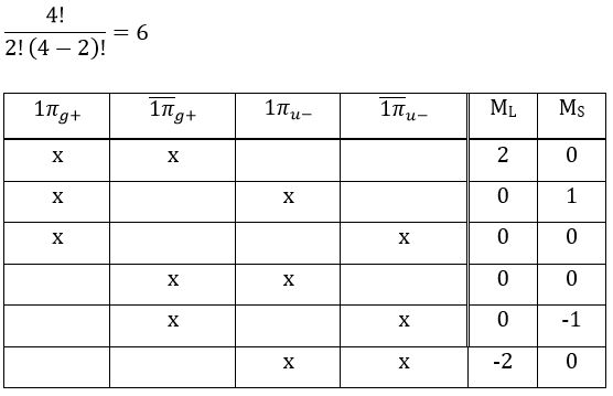
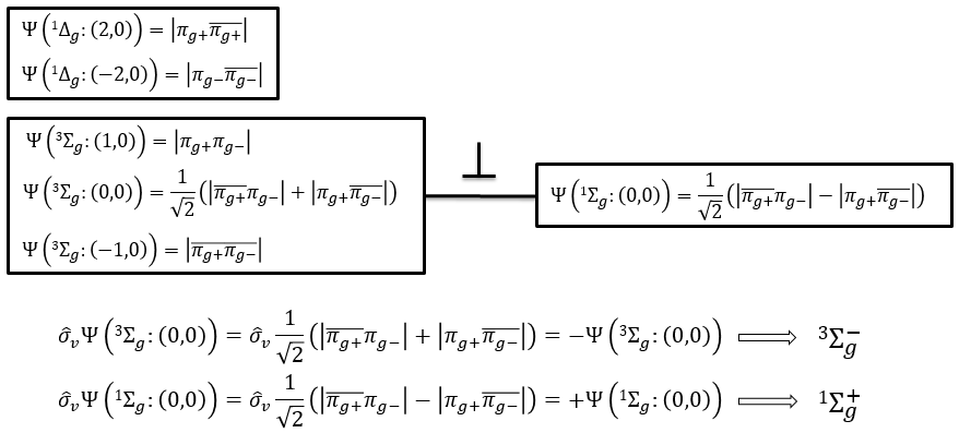
The first emergent is (2,0). That corresponds to the group 1Δg. Remember that the degeneration for linear molecules is 2 except for ML=0. In the atomic case, we had a degeneration of 2L+1 (i.e. ML, ML-1, …, 0, …, –ML-1, -ML) but here we just have ML and –ML. The next emergent is (0,1), a triplet 3Σg. Finally there is a singlet 1Σg. To know if it is Σ+ or Σ–, we have to apply the operator σv. In this case we have 3Σg– and 1Σg+.
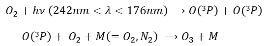
Ozone is obtained by the excitation of one molecule of O2 at its fundamental state into two oxygen atoms in the 3P state. In this state, they react with another molecule of O2 and a catalyst to produce the ozone.
Chapter 3 : MPC – Group’s theory
Because of the particular geometries of some molecules, the CSCO may be different. Instead of the CSCO that we had with the atom, we want to determine the CSCOH: the complete set of operators commuting with Ĥ. It is thus a set larger than the CSCO because the operator don’t have to commute between them. The CSOCH can be subdivided into groups (SCO) of similar operators but they do not necessarily commute between each other.
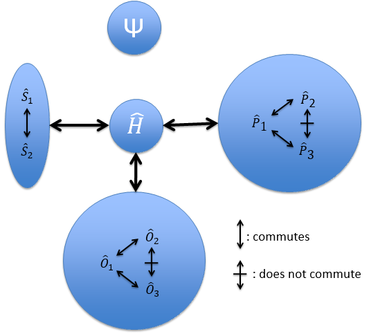
When two operators of the CSOCH don’t commute together, it implies a degeneration of the states.
In the case of atoms, when we have a spherical symmetry (it has been shown recently that some atoms are slightly deformed and have an elliptic shape (and then a quadrupole moment) or a pear shape (and then an octupole moment)), we have the usual CSCO. We can build 3 SCO:
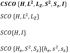
This last group is present for any system of electrons: the spin of the electrons is independent of the geometry of the molecule. The small letters correspond to operators of orbitals. In the case of a linear molecule, we lose the spherical symmetry but there is still a cylindrical symmetry. Instead of an infinity of axis of rotation passing by the nucleus, we have now only one axis of rotation on the axis of the two (or more) nuclei. This difference induces a modification of the SCO’s: we lost the L2 symmetry. As reminder, L2=Lx2 + Ly2 + Lz2. LZ is still in the SCO but Ly and Lx are not anymore commuting with H. We have now
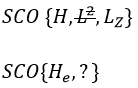
In the case of nonlinear molecules, we also lose the operator LZ.
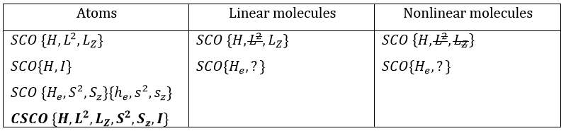
We have other symmetry operators that we have to add to the CSOCH (showed by the ? above):
- a bilateral symmetry σv: there is an infinity of planes of symmetry passing by the axis of the molecule.
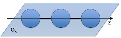
- a centre of inversion Î if the linear molecule is centro-symmetric (same atoms at each side of the centre of the molecule, ex: CO2, N2, C2H2).
Those operators are necessary to describe completely the molecule: the operators of symmetry characterise the spatial behaviour of the system. As a result, the ensemble of all the operators that commute with H define the state of the system from the spatial point of view. If we forget some operators in the CSOCH, one part of the quantic information is lost. We say that the ensemble of the operations of symmetry form a mathematic group.
Theory of groups
G={a, b, c, …} forms a mathematic group with regards to one law (*) if
- * is intern and defined everywhere: a*b=c a, b, c ϵ G
- * is associative: (a*b)*c=a*(b*c)
- ∃ e neutral (e ϵ G) : a*e=e*a=a
- Reversibility: ∀ a, ∃ x=a-1 ϵ G : a*a-1=e.
For a group of symmetry, a*b means that we apply the operation b first then the operation a.
The order h of a group of symmetry G is the amount of operations it contains. A group of symmetry can be continuous (order h of G is infinite, i.e. a symmetry of revolution) or finished (h is finite), commutative (or abelian) if a*b=b*a ∀ a and b ϵ G, or non-abelian (what leads to a degeneration).
The representation of a group is a set of n by n matrices (n being the dimension of the representation) {D(a), D(b),…} associated to the elements {a, b, …} of G such as
- the matrix product is associated to the law (*)
- the matrix unity is associated to the neutral e.
The representation is said to be reducible if the matrices can be diagonalised and irreducible if it is not the case. Any reducible representation D of G can be expressed as a linear combination of the irreducible representations Di of G.
![]()
We can thus search for the operators of symmetry of a molecule that let the Hamiltonian unchanged. It is the interactions electron-nucleus that impose this symmetry.
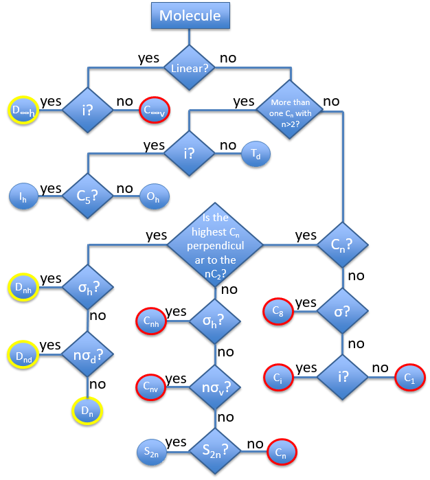
There are 5 operations of symmetry:
- identity: E – no displacement
- inversion: I – central symmetry or centre of inversion
- reflexion: σv(vertical) σh(horizontal), σd(diedre) – planar or bilateral symmetry
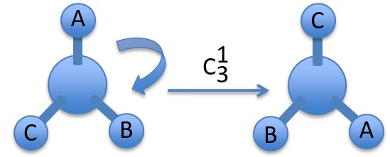
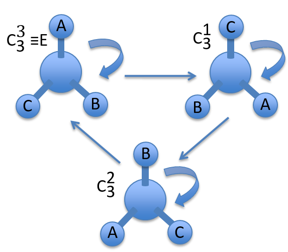
- proper rotation: Cn – rotation of 2π/n rad around the axis
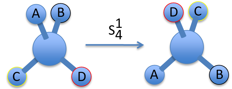
- improper rotation: Sn – commutative product of a rotation of 2π/n around the axis with a reflexion in the plane perpendicular to the axis.
To apply several consecutive rotations we add an exponent x to Cn or Sn. It means that we apply the rotation 2π/n x times. x goes from 0 to n for Cn and up to 2n for Sn. The Some elements are equivalent. For instance C33=E
The groups are named following this picture:
Now lets come back quickly on the properties of the groups.
Faire pareil: d’abord expliquer avec les opérations sur la base 3 puis dire que pour l’explication il était plus simple de montrer avec les axes x,y,z mais qu’en réalité, en utilisant d’autres coordonnées on arrive à une représentation de dimension 4 qui donne lieu à une ligne supplémentaire.
Let’s take a look on how we build the representation of the group of symmetry C2V, i.e. the group of shouldered molecules as H2O, NO2 but also as CH2O. If we draw H20 in the Cartesian coordinates such as
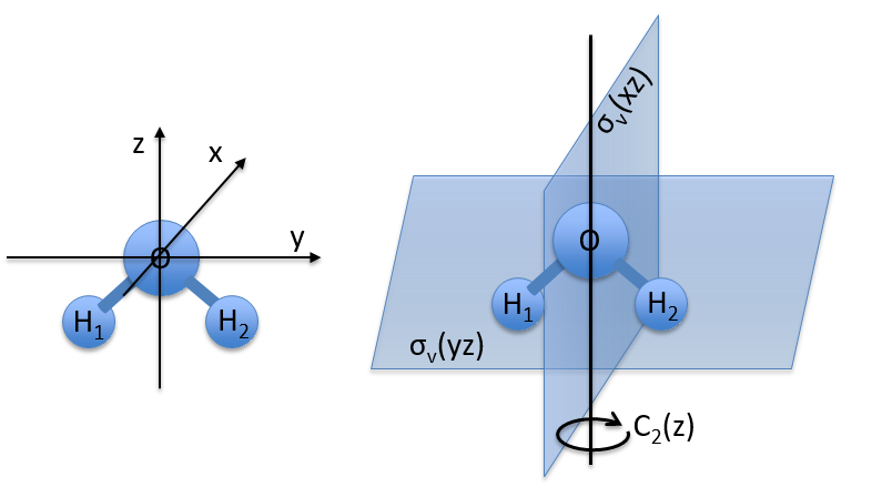
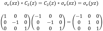
If we apply an operation of symmetry on the molecule, for instance σv(xz), i.e. the reflexion in the plane xz, the molecule did not change but if we follow one of the hydrogen atoms, its coordinate y changed of sign ((x,y,z)à(x,-y,z)). We can translate this into a matrix of dimension 3 that we apply on the coordinates x, y and z:
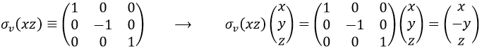
Such a matrix can be found for the other operators of the group
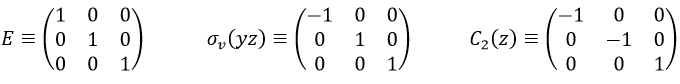
These matrices commute together and the group is intern and defined everywhere. For instance
Each column of the representation of the group is the value on the diagonal of the matrix for the corresponding base (here the coordinates x, y, z)
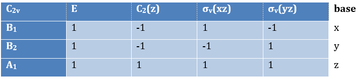
Those values are associated with the quantic numbers and the parity. 1 means symmetric and -1 antisymmetric. The character of one matrix associated to the operation a is the sum of the elements on its diagonal and is noted χ(a).
![]()
Let’s come back to something we said earlier: any reducible representation D of G can be expressed as a linear combination of the irreducible representations Di of G.
![]()
The coefficients can be determined from the characters of the matrices associated to the operations of this group because of the properties of orthogonality.
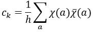
Where χ ̅(a) is the value of the irreducible representation associated to one base. For instance, in the base A1 we have χ ̅(E)=1, χ ̅(C2(z))=-1, χ ̅(σv(xz))=1, χ ̅(σv(yz))=-1
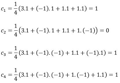
Applied to the C2v group, it gives
![]()
We will see next that there is in fact a fourth line (A2) in the table and why it is necessary to correctly describe molecule.
And thus
![]()
A group is normed if its order h, equal to the amount of operations, is also equal to the sum of the squares of χ ̅(a), and this for each irreducible representation, i.e.
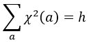
For C2v, h=4=12+12+12+12 (in the case of the operation E). For the operation C2(z) we find the same value: h=4=12+12+(-1)2+(-1)2. Two representations k and l are orthogonal if
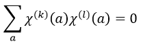
For instance, we obtain for A1 and B2
![]()
The group C3v describes molecules such as NH3. It contains 6 operations: E, two C3 and three σv. We can represent it as
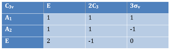
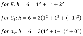
The irreducible representation E is degenerated: it contains a value different from -1,0 or 1. Yet the group is still normed (don’t forget there are two C3 and three σv):
The representations are orthogonal (for instance between A1 and E):
![]()
Application of the theory of groups
Each orbital of the atoms of one molecule is a basic function that impacts the geometry of the molecule. We need all of those functions to describe correctly and completely the molecule. As a result, a molecule such as NO2 is described by one representation of base 15 that can be reduced into 10 complete bases (5 of dimension 1 for the nitrogen and 5 of dimension 2 for the oxygen) because the two oxygen atoms are equivalent.
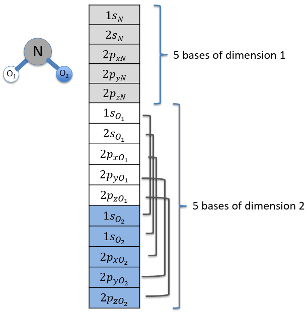
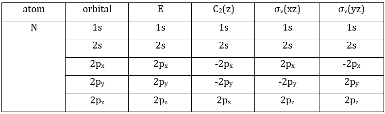
We have seen previously that the NO2 molecule belongs to the group of symmetry C2v. If one representations of N can be transformed by one operator of this group into itself in absolute value, it means that this representation is an irreducible representation of the group for the atom N. It is indeed the case for NO2:
- all of the orbitals of N are irreducible: the orbitals s are spherical so the operation of symmetry changes nothing while the orbitals p change of sign for some operations of symmetry.
- the orbitals of the oxygens are transformed into themselves or into an orbital of the other oxygen, in absolute value.
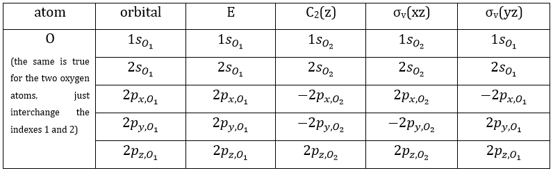
We can thus find a matrix D(R) such as when it is applied to the base we find the linear combination that belongs to the group.To build a representation of the group C2v, we have to build one matrix of dimension n for each operation of symmetry of the group, i.e. 4 matrices. Those matrices define the transformation with regard to the four operations of symmetry of one base of n functions. The base has to be complete, i.e. the action of one operation on one of the functions of the base has to give a linear combination of functions of the base. In mathematical words,

The set {D(R), D(R’),…} is a representation of the group G.
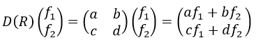
The trace T(R) is the sum of the diagonal members of the matrix D(R) (here it is a+d). The set {T(R), T(R’),…} characterises the representation of the group D.
From a few irreducible representations of one group, we can find the other representations of the group. We proceed that way:
3 representations can be found from the nitrogen (see the table behind). One representation (A1) is when none of the orbital changes during any operation of symmetry. This representation works for the orbitals 1s, 2s or 2pz. A second representation (B1) stands for the orbital 2px for which C2(z) and σv(yz) change the sign of the function. The third representation (B2) is when C2(z) and σv(xz) change the sign of the function, i.e. in the case of the orbital 2py.
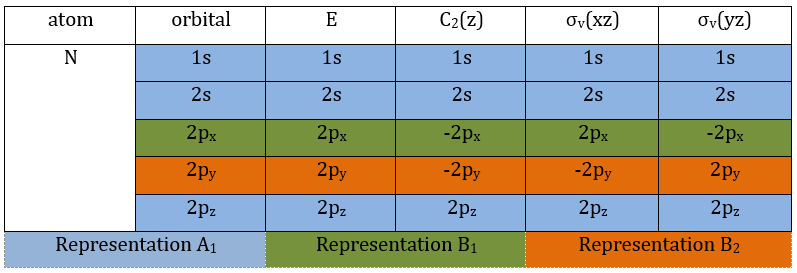
We can write the representations in a table
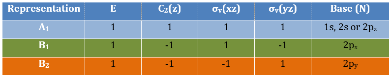
These three representations are not the only ones that apply to the NO2 molecule. We must also describe the orbitals of the atoms of oxygen to give a complete description of the molecule. In this case, it is a bit more complicated because the operations of symmetry can transform one oxygen into itself or into the other oxygen, in absolute value. As a result, the representation is not a series of numbers but a series of 2×2 matrices. If the orbitals remains unchanged by an operation, the matrix corresponding to this operation of symmetry is
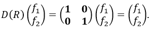
If the atoms are interchanged, the matrix is
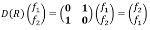
and if the sign changes it is
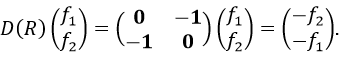
For instance, D(E) of the 1s orbitals is (1 0 sur 0 1) because
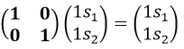
The operator σv(xz) interchanges the atoms of oxygen: and D(σv(xz))=(0 1 sur 1 0) because
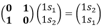
And we can do that for the other operations as well. That being done, the table of the group C2v is completed:
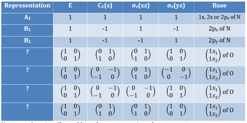
However, there is still a problem: the representations that are matrices are not irreducible. But we can find from which linear combination of irreducible representations they come from the traces of the matrices.

One can see that we can combine the representation A1≡{1 1 1 1} with the representation B2≡{1 -1 -1 1}. The representation corresponding to the base (1s1, 1s2) is thus A1 + B2. We can repeat this process for the other bases of the group. It works fine for 3 bases but not for the base (2px1, 2px2). There is thus an unknown representation A2 in the group so that we can build the matrices of the base (2px1, 2px2). Obviously the combination will involve the representation B1 to obtain a trace of -2 for the operation σv(yz). The representation A2 is thus A2≡{1 1 -1 -1}.

If you remember well, earlier in the course we discussed on the operators of symmetry of the water and we already talked about a fourth representation in the group C2v. Now you know why we needed this fourth representation. It is required to build the CSCO that would not be intern without A2.
Amongst the 15 atomic orbitals of NO2, we have 7A1 + 1A2 + 2B1 + 5B2:
7A1: 1s, 2s, 2p, (1s1,1s2), (2s1, 2s2), (2py1, 2py2), (2pz1, 2pz2)
1A2: (2px1, 2px2)
2B1: 2px, (2px1, 2px2)
5B2: 2py, (1s1,1s2), (2s1, 2s2), (2py1, 2py2), (2pz1, 2pz2)
To build the representation A1, we will thus need a linear combination of the 7 orbitals.
Method of projection
The projection allows to determine which orbitals take part to which representation. In a general way, the operator of projection P(i) for non-degenerated representations is given by
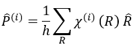
with i the corresponding representation, χ the trace of the operator and h the norm. For instance, applied to NO2,
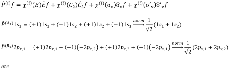
To obtain π liaisons, the p orbitals have to be oriented correctly. On the other hand, antibonding liaisons are the result of p orbitals that are (also) correctly oriented but with opposed signs. We know that there are 3 unoccupied orbitals in NO2 (15 orbitals and 23 electrons). These orbitals are some of the antibonding orbitals and are the highest in energy.
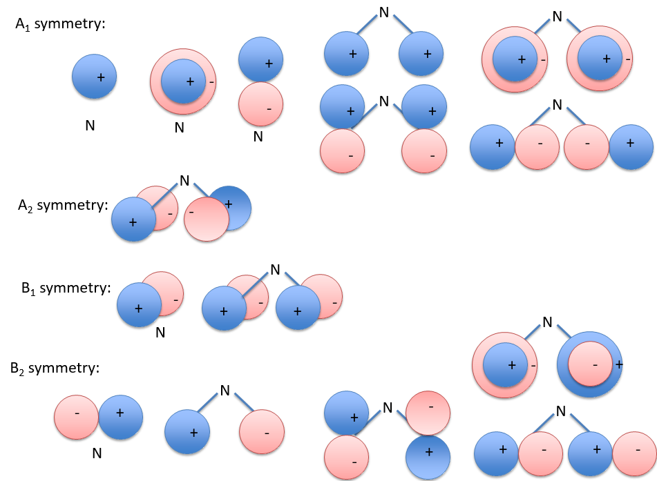
For degenerated representations, we can still do the projection using the diagonal elements of the matrix D(i). The formula changes a bit:
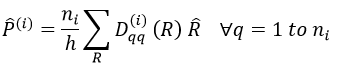
with ni the degree of degeneration.
Application to NH3
NH3 belongs to the C3v group.
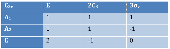
Obviously the presence of a 2 in the irreducible representation E indicates that this IR is degenerated. The orbitals to consider are
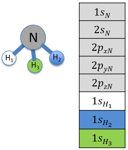
The orbitals s of N belong to A1 because they are spherical and the 2pz also does because it is on the axis of rotation. The rotations that we can apply on NH3 are of 120°, so our system of coordinates is not very convenient here. We can however obtain the matrix representation of {2px, 2py}
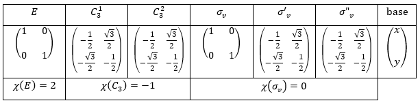
The matrix representation of {2px, 2py} is thus the irreducible representation E: the traces of the matrices correspond to the elements of the IR E in the table of C3v.
We repeat the process for the three hydrogen atoms
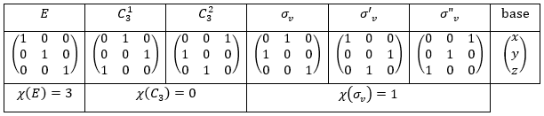
It doesn’t correspond to any IR of the table C3v but we can find a linear combination of them:
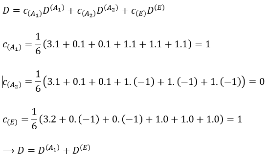
There are two projections for the operation E as it is degenerated twice. The atomic orbitals adapted to the C3 symmetry are, for the hydrogen atoms
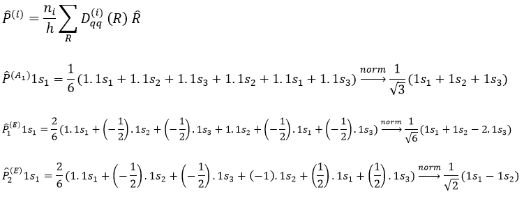
We already verified the orthogonality of C3v previously
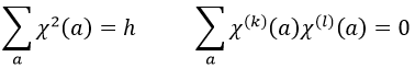
Proper functions
The proper functions of Ĥ (polyelectronic states) and of ĥ (molecular orbitals) that have a proper value E in common form a base for the irreducible representation of G.
Non-degenerated case:
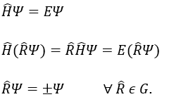
We can thus reduce the molecular representation of dimension n into n matrix representations of dimension 1.
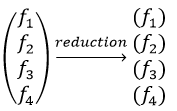
Degenerated case (n times):
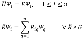
Several proper functions have the same energy. As a result, the reduction leads to several representations amongst which some are not of dimension 1.
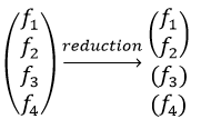
Direct Product of two representations
The direct product between two representations of dimensions n and m give a n.m representation. It allows to determine the symmetry of the product of two or more representations, i.e. in case of coupling between orbitals. For instance, the direct product of one representation D(1) of base f (dimension n1=3) with one representation D(2) of base g (dimension n2=2) gives a representation D of base fg (dimension n=n1.n2=6)
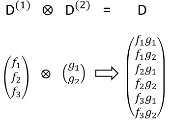
The character of the new representation will simply be the product of the characters of the old representations (no need to do all the stuff).
![]()
We can thus determine the symmetry of the product of several functions.
The direct product with one 1D representation gives an irreducible representation. If the representation is reducible, it is a linear combination of the representations of the group.
Most of the molecules have a fundamental state that is an A1 representation because the octet rule is respected. I understand that the direct product and its interest are vague for now but we will see them with the example of NH3.
Example of NH3
NH3 belongs to the group of symmetry C3v.
The direct product of two E representations gives in the group C3v gives
![]()
This product corresponds to a linear combination of the IR of the group.
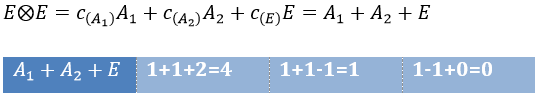
The coefficients can be determined from the relation
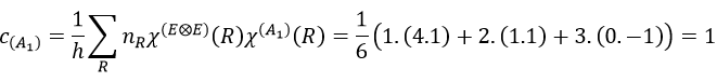
The molecular orbitals are called in function of their irreducible representation, written in small letters. The fundamental state of NH3 is
![]()
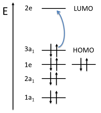
The MO 1a12 results from a coupling between two A1 states: A1xA1=A1. It is the same for the other a12 molecular orbitals. For the 1e4, we have the coupling of 4 E representations. The E representation is of dimension 2 and the coupling gives a degeneration of 16 (24). However, the principle of Pauli has to be respected as well, i.e. the only possibility is that the 4 electrons are distributed amongst the two orbitals of same energy with opposite spins. As the layer is full, the representation is A1.
If one electron of the HOMO (orbital 1e4) is excited to the orbital 2e (LUMO) we obtain two 2E states (1e3 and 2e1 give the same state by the symmetry hole/particle).
![]()
Cases of the spherical and cylindrical molecules (or atoms) – group of symmetry Kh
I don’t know the exact reason, but for those two cases the representations have specific names. For atoms, the representations have names identical to the atomic symmetry. The orbitals s belong to the group S (dim 1), the orbitals p belong to the group P (dim 3), etc. We can put an index to the group that translates the parity in this group. The index is g (gerade from German) if the state is symmetric and u (ungerade) if the state is antisymmetric.
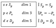
If we apply the inversion operator on the nitrogen, we have
![]()
The coupling between two identical indexes gives gerade and between two different indexes gives ungerade:
![]()
The groups for linear molecules that are not centrosymmetric are called differently
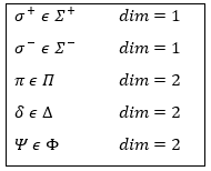
The distinction between σ+ and σ– is the direction of the rotation (clockwise or anticlockwise).
For centrosymmetric molecules, we note the distinction between ungerade and gerade
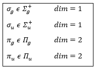
Chapter 2 : MPC – Molecules and Born-Oppenheimer
The Hamiltonian quickly becomes monstrously difficult when several atoms and electrons are considered. To illustrate this point, the equations of the Hamiltonians for H, H2+ and H2 are showed below:
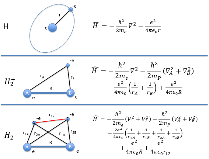
For a molecule with M nuclei of atomic number Z1, Z2, Z3, …, ZM and n electrons, the global expression is
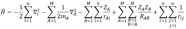
The Hamiltonian can be decomposed into 5 terms, two from the kinetics of the electrons and nuclei and 3 for the interactions between the electron-electron, nucleus-nucleus and nucleus-proton.
![]()
As soon as there are several nuclei, there is no central field anymore and we can’t develop a spherical symmetry to build the CSCO. To simplify the problem, we use the Born-Oppenheimer approximation. The electrons have a mass that is way smaller than the one of nuclei (around 1800times smaller than the mass of a proton) and they move way faster. The approximation is to consider that the electrons are adapting themselves instantly to the movements of the nuclei and that we can consider the nuclei as immobile to determine the movements of the electrons.
As a result, we get one equation of Schrödinger for the electrons in the field of the fixed nuclei (TN=0).
![]()
The coordinates of the nuclei are a parameter and not a variable anymore in this equation. We can solve the equations for any position of the nuclei. Then we solve the Schrödinger’s equation for the nuclei.
We treat a single electronic state at a time. It gives the surface of potential energy. We talk about a surface of potential energy but the dimension depends on the quantity of nuclei. The surface of potential energy depends on 3M-6 intern coordinates) (3M-5 for linear molecules) where M is the amount of nuclei. The -6 comes from the fact that the 3 degrees of translation and of rotation do not impact the potential energy. The global wave function of the molecule is the combination of the wave functions for the electrons and the nuclei. We can plot the potential of BO simply by the addition of the electronic energies as a function of the distance between the nuclei with the nucleic potential.

It forms the potential of Born-Oppenheimer that can show a minimum and the state is binding, or no minimum and the state is not binding: the most stable distance between the nuclei is infinite.
During a reaction, the distances between the nuclei vary to form a new liaison and we can plot isocurves of potential energy as a function of the internucleic distances but the approximation that the nuclei are immobile becomes bad as their movements are an important parameter of the problem. It is the case during the cleavage or the formation of a liaison.
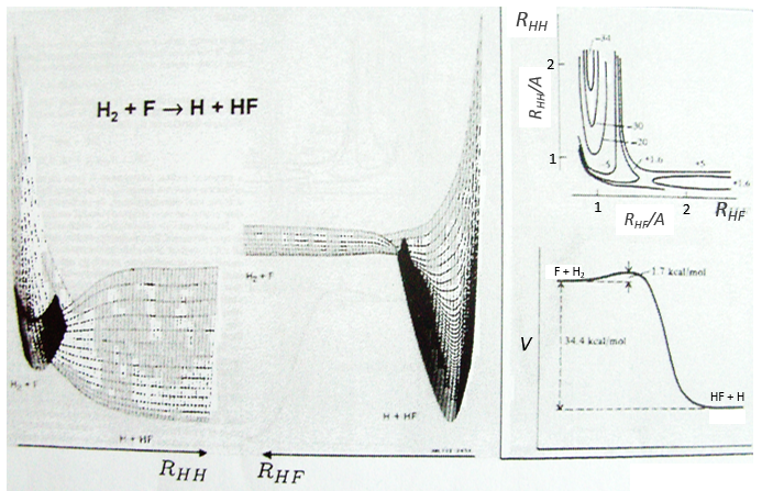
Something that was neglected in the approximation of BO is that the different states can interact together and that the couplings between these states can be important. We isolated one state and neglected the couplings it can have with the other states. The exact solution takes them into account. The difference is especially important if two states are close in term of energy or if there is a crossing of the states of energy as a function of the distance between the nuclei (see below an example for the diazomethane, the parallel lines are for various angles of approach). In these cases the coupling terms are not negligible anymore and the approximation.
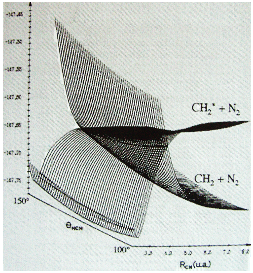
Chapter 1 : MPC – polyelectronic atoms
The presence of a second electron induces a term of repulsion between electrons.
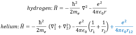
This term is positive so it increases the energy of the orbitals. The rest of the equation is similar to the Hamiltonian of the hydrogen. We can compare the energy of the orbitals with those two models.
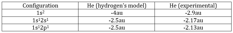
The repulsion is large in the 1s orbital wherein the electrons are close to each other (the radius being small). For instance, the energy of the orbital 1s2 of the Helium is at -2.9au (atomic units). If we calculate the energy without the repulsion term, i.e. as a monoelectronic atom (Ĥ= Ĥ1 + Ĥ2), we find -4au (E1=E2=-Z2/2n2=2au). Another consequence is that the orbitals s and p don’t have the same energy anymore. The configurations 1s12s1 has an energy of -2.17au and the configuration 1s12p1 an energy of -2.13au.
We can separate the Hamiltonian into one monoelectronic Hamiltonian term and the term of repulsion between the electrons.
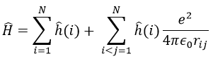
ĥ(i) is the monoelectronic Hamiltonian of one electron. We sum up the terms for all the electrons to obtain the Hamiltonian. To resume, the repulsion spreads the degenerated orbitals from the monoatomic model.
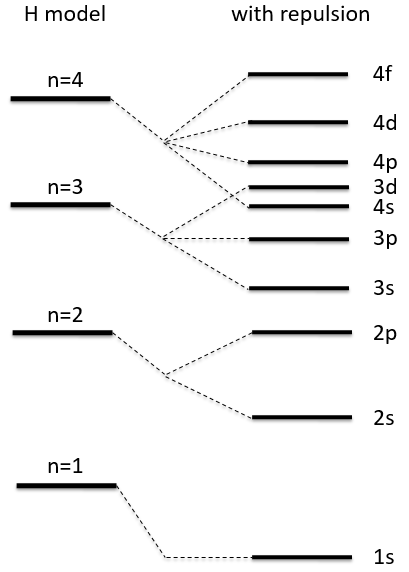
The repulsion can be large enough to have an orbital of level n+1 of lower energy than an orbital of n. It is the case for orbitals d and f and it is why we use the following technique to fill the orbitals with electrons:
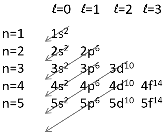
The 4s orbital is thus filled before the 3d orbital.
The operators that commute are simply the sum of the operators applied to the electrons independently (but perturbed by the repulsions). We write these operators with a lower case to denote them from the global operators (Ĥ→ĥ, Ŝ→ŝ, …).
The electrons are indistinguishable. It means that if we exchange an electron of an atom with another electron of the atom on the same orbital or on a different orbital, the atom remains unchanged. We can thus introduce a permutation operator Pij that commutes with the Hamiltonian Ĥ and the proper value of which is ±1. This last affirmation is true because we get back to the initial conditions if we apply the permutation operator Pij twice. The identity operator Ê is the operator with which nothing changes: ÊΨ=Ψ.
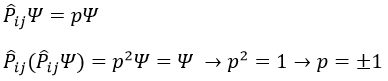
The value of p is imposed by the type of particle. Bosons have a integer spin and pboson=1. Fermions have half-integer spins and pfermion=-1. Electrons are thus fermions. Some nuclei are bosons and some are fermions. In an atom with N electrons, N! permutations of electrons are possible. For instance, the lithium has 3 electrons with spherical coordinates (r1, σ 1), (r2, σ2) and (r3, σ 3) (considering the orbitals 1s and 2s) that can be permuted between 3 spots a, b and c. There are 6 possible permutations 6=3! = 3x2x1): P12, P13, P23, (P13,P12), (P13,P23) and Ê.
We don’t know which electron is in which spot (a, b or c). The wave function Ψ is one of the functions
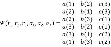
To write the wave function we use the determinant of Slater which is a combination of the possible states.
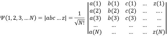
with a, b, c, …, z are the spin orbitals.
In mathematics, a determinant is read in diagonal. The elements of the diagonals (from top left to bottom right) are multiplied and the diagonals are summed up. Then we deduce the diagonals in the other way (from top right to bottom left). In the case of the lithium we have
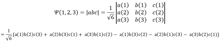
The determinant of Slater has a few properties:
- if we exchange two lines or two columns, the sign of the determinant changes.
- if two columns are identical, the determinant equals 0.
It can be translated by the law of Fermi: 2 electrons must differ by at least one quantic number.
Let’s apply this to the helium and a few of its excited states. He has 2 electrons that are distributed on the 1s orbital in its ground state. There can be two electrons on this orbitals if they have different spins (1/2 and -1/2). In the notation of Slater, the spin is indicated by the presence of a line above the orbital if the spin=-1/2.
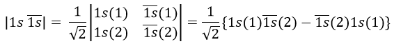
For the excited state wherein one electrons jumped to the orbital 2s, there are 4 possible states depending on the spin of the electrons:
![]()
For instance,
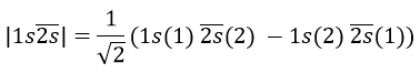
If instead the electron jumped to the 2p orbital, there are 12 possible states:
![]()
For instance,
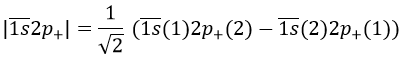
Coupling of Russel-Saunders
This coupling is also called the L-S coupling. We consider it for multi-electron atoms with weak spin-orbit couplings. In this case, the orbital angular moments of the individual electrons add to form a resultant orbital angular momentum L and the same is true for the spin moments to form a spin angular moment S. L and S combine to form the total angular moment J.
J=L+S
The resultant of two vectors is their sum. If we consider two operators Ĵ1 and Ĵ2 (which can be L and S), their resultant Ĵ = Ĵ1+ Ĵ2.
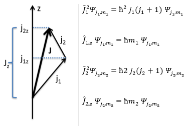
Ĵz is simply equal to the sum of Ĵ1z and Ĵ2z and Ĵ2 is the development of the square of the sum
![]()
We can look at the coupling between the electrons in He. The electrons have a spin s=1/2 and ms=±1/2. Let’s say that ms=1/2 is the state α and that ms=-1/2 is the state β. The coupling can be αα, αβ, βα or ββ coupling. The coupled Ms=ms1+ms2 can thus be equal to 1, 0, 0 or -1. We write these values in a table. I insist on the fact that Ms=0 is degenerated.
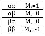
To know the resulting states of the coupling between the electrons, we take the largest S=s1+s2 and look for its Ms in the results of the coupling. It is Smax=1 with Ms=-1, 0 and 1. We discard these values of Ms from the 4 couplings that we obtained earlier. If there are one or more remaining Ms in the table, we do the same for S=Smax-1, etc. Here, there is one last Ms=0 that comes from S=0. The 4 couplings correspond thus to a singlet state (S=0 and Ms=0) and 1 triplet state (S=1 and Ms=1, 0 or -1). S goes from ∣s1+s2∣ to ∣s1-s2∣ by step of 1. The multiplicity is equal to 2S+1. The difference between the states is always by step of ΔS=1 and ΔMs=1. The states can be represented this way:
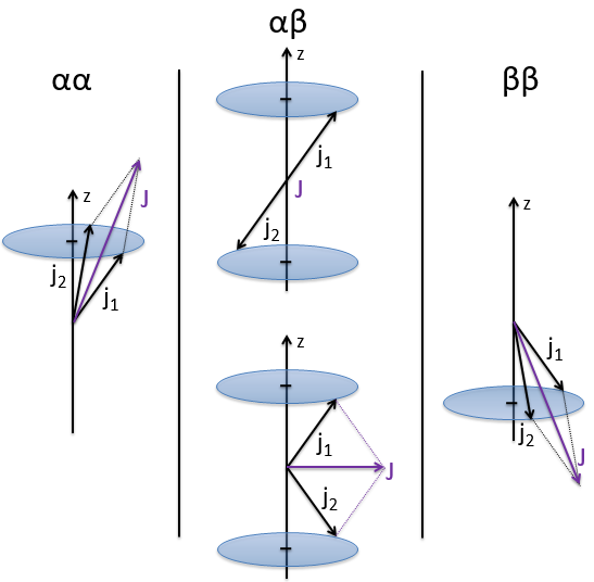
Note that the vectors for Ms=1 or Ms=-1 are not two times the length of the vectors for ms1 and ms2. The vertical component is. Note too that the resulting vector for Ms=0 may have a nonzero length (S=1).
If 3 electrons are coupled, we proceed step by step. First we do the coupling between two electrons. As previously we obtain two different states, S12=0 (singlet) and S12=1 (triplet). There is no need yet to determine Ms. The last electron is coupled next to the two possible states S12. The coupling with the singlet S12=0⊗s3=1/2 gives S123=1/2. It is a doublet (Ms=1/2 or Ms=-1/2, remember that ΔMs=1 between ∣S12+s3∣ to ∣S12-s3∣). The coupling S12=1⊗s3=1/2 gives a total of S123=3/2 (1+1/2), leading to two states S123=3/2 and S123=1/2 (ΔS=1). It means that there is a quadruplet (2(3/2)+1=2) and a doublet (2(1/2)+1=4). In total, there are 2n=8 possible states, n being the number of electrons.
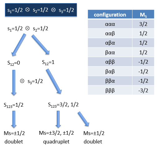
In the case of degenerated orbitals as the orbitals p or d, the amount of configurations is larger (see the part about the determinant of Slater) but the method is identical and is also applied to the quantic number l. Let’s take a few examples: the electronic configurations (1s)1(2s)1, (1s)1(2p)1 and (2p)1(3p)1.
Configuration (1s)1(2s)1
The degeneration is 4: the two electron can have a positive or a negative spin (α or β). We have thus 2×2=4 degenerated configurations:
![]()
There is only one value for the orbital number L=0: l1s=0⊗l2s=0. As a result, ML=0. As we have seen above, the coupling between two electrons s1S=1/2⊗s2s=1/2→S=1, 0 gives one singlet (S=0, degeneration =1) and one triplet (S=1, deg=3).
We write the electronic term depending on L and S. L gives a capital letter S, P, D, F the same way n gives s, p, d, f. The electronic degeneration is written as an exponent before the orbital letter. The electronic terms for the configuration (1s)1(2s)1 are thus 1S, 3S. The degeneration of the terms is the multiplication of the degeneration of L and S and we sum up the degeneration of the electronic terms: 1.1 (for 1S) +1.3 (for 3S) = 4. We have thus a concordance between the degeneration of the terms and the degeneration of configuration.
Configuration (1s)1(2p)1
The degeneration is 12 in this case: both electrons can have a positive or negative spin (α or β) but the 2p electron can be on 3 different orbitals (2p–, 2p0 or 2p+). We have thus (1.2).(3.2)=12 degenerated configurations (written earlier in the chapter).
The coupling l1s=0⊗l2p=1 gives L=1 (ML=-1, 0, 1). There is no L=0 here: if we look at the details of the coupling.
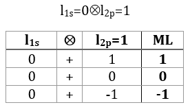
We find the ML’s of L=1 but once they are discarded, there is no other ML. There is thus no L=0. An easier way to know it is that L goes from ∣l1=l2∣ (=1) to ∣l1-l2∣ (=1-0=1).
As L=1, the electronic terms will be xP with x=1 and 3 from the spin. As always, the coupling between two electrons gives a triplet and a singlet. The electronic terms are thus 1P, 3P with a degeneration (3.1)+(3.3)=12.
Configuration (2p)1(3p)1
The degeneration is 36 ((3.2).(3.2)): 3 orbitals with 2 possible spins for each electron. The coupling l2p=1⊗l3p=1 gives L=2 (ML=-2, -1, 0, 1, 2), L=1 (ML=-1, 0, 1) and L=0 (ML=0). The coupling of spins gives one singlet and one triplet as usual. We have thus the electronic terms
1S, 1P, 1D, 3S, 3P, 3D that can also be written as 1(S, P, D), 3(S, P, D) or even 1,3(S, P, D)
The degeneration are respectively (1.1), (3.1), (5.1), (1.3), (3.3) and (5.3) for a total of 36.
If we want to couple a third electron, we obtain the electronic terms by coupling separately the electronic terms if the electrons are not equivalent. For instance, if we add a 3d electron (2D) to the 2p3p electrons, we proceed this way:
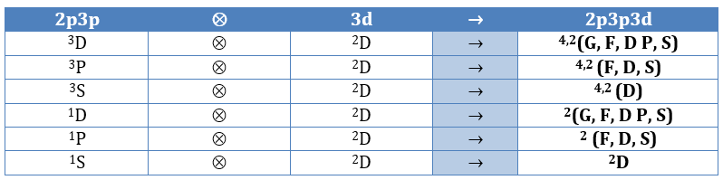
One can see that some electronic terms are obtained several times (2F for instance). Those terms are not identical and have not the same energy because they come from different couplings.
In the case of equivalent electrons, the amount of states is more limited. For instance we had 36 possibilities for the 2p3p configuration. This amount drops to 15 for the 2p2 configuration. This amount is equal to X!/(X-N)!N! where X is the degeneration of the state and N the number of electrons. In our case, 2p2, N=2 and X=6 for the orbital 2p: there are 3 orbitals (2p+, 2p0 and 2p–) and 2 spins. There are thus 6.5/2=15 possibilities. To determine the electronic terms of this coupling, we will make a list of the 15 possibilities and identify each one by the couple (ML,MS). To do so we draw a table with a column for each one of the 6 states and we put pairs of electrons together. In a seventh column, we write down the (ML, MS) of the couple of electrons.
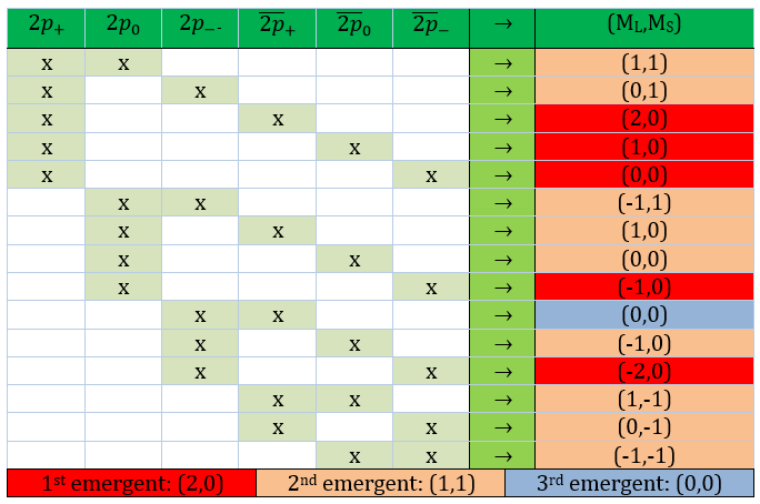
Once it is done, we seek for the emergents. An emergent is one couple of projections that is unique. We take the one with the largest values, i.e. (2,0) in this case and we determine the electronic term from which the pair comes. ML=2 means that L=2 and MS=0 means that S=0. The corresponding electronic term is 1D that has a degeneration of 5. As a consequence we will find 5 pairs of projections in the table that come from the electronic term 1D.
We can remove them from the list and look for another emergent: (1,1). The corresponding electronic term is 3P with a degeneration of 9. From the 15 possibilities, 14 correspond to 2 electronic terms (3P and 1D). The last emergent is (0,0), what corresponds to the electronic term 1S. The electronic terms of the configuration 2p2 are thus 1D 3P 1S. In comparison with inequivalent electrons (2p3p), the 3D, 1P and 3S terms disappeared. Also note that several pairs were several times in the list and we randomly selected which one corresponds to which electronic term. For instance, we don’t know which (1,0) comes from 1D or from 3P.
In terms of energy, the rules of Hund tell us that the term with the highest MS is the most stable. If there are identical MS projections, then the highest ML is the most stable. For instance, the 3P coupling of 2p2 has a lower energy than 1D itself lower than 1S.
Here come two properties of the L-S coupling:
- Complete orbitals are all 1S:
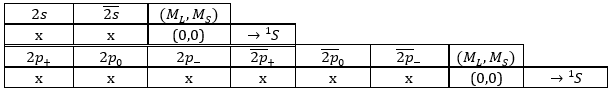
As a result, they do not modify the other orbitals. Note that even if they do not perturb the other orbitals, they do contribute to the energy of the electronic states.
- A “hole” (the absence of electron) in one orbital gives the opposite signs of ML and MS than the presence of this electron. For instance
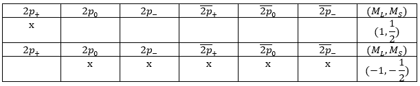
But the sign doesn’t change the state. As a result, the carbon (2p2) and the oxygen (2p4) have the same state 2P.
Spin-orbit coupling
The magnetic moment induced by the spin of the electron interacts with the magnetic field induced by the electric current resulting from its orbital movement. This relativist effect induces a further separation of the states and an additional term in the Hamiltonian.
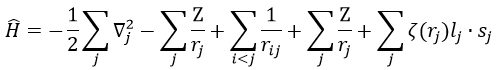
The coupling introduces a new observable J=L+S
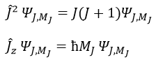
J goes from L+S to ∣L-S∣ by step of 1. Considering this, [Ĥ,L2] and [Ĥ,Ŝ2]≠0 but [Ĥ,Ĵ2]=0.
The relativist effects grow with the atomic number of the atom: the larger the atomic number, the heavier the nucleus. Its charge increases as well meaning that the electrons have to revolve faster to compensate.
Energy of the states
The energy of the states can be found from the equation of Schrödinger
![]()
From that, we can write
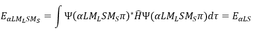
The energy is thus the average value of Ĥ. To determine it, we start from a linear combination of determinants of Slater (ML,MS). An emergent determinant of Slater always gives a proper function. From this point, we can apply operators L+, L–, Ŝ+ or Ŝ– to increase/decrease the value of ML or MS and find their energy.
![]()
We do it for each state that has at least an emergent. If there is no emergent, we can apply the rules of orthogonality: 2 wave functions that differ by at least one proper value of operators that commute together are orthogonal. Eventually, the proper functions are normalised.
With this method, the energies of the states can be found. One simple example says more than a thousand words. The coupling of two electrons gives a singlet (S=0, MS=0) and a triplet (S=1, MS=1, 0, -1). We will place the values of MS in boxes for S=1 and S=0, as shown below.
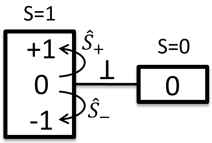
An emergent is found for MS=1 (S=1) so we can find the wave function ΨS=1,Ms=1 (the state αα). We also have the wave function of Ψ1,-1 (the state ββ) because it is an emergent too.
To obtain the wave function of the state MS=0, we apply the operator of descent Ŝ– on Ψ1,1 (we could have applied Ŝ+ on Ψ1,-1 instead).
![]()
One electron in the α state is thus now in the β state. We need to norm the function. To do so, we must have the norm N equal to
Applied here, we have
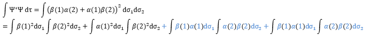
The orbitals are orthonormal, meaning that the integrals equal 1 if the two terms of the integrant are identical and zero if they are different: ∫αα=1, ∫ββ=1, ∫αβ=0, ∫βα=0. The cross terms of the square (in blue) are thus equal to zero and the others equal 1.
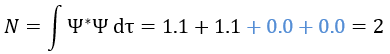
As a result,

To obtain the wave function of the singlet, we can use the property of orthogonality between Ψ1,0 and Ψ0,0. Posing β(1)α(2)=x and α(1)β(2)=y,
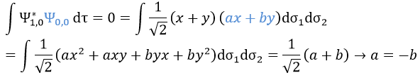
Meaning that, once normed,
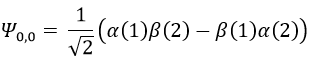
The same method can be applied on more complex cases. For instance with two 2p electrons: